


The Nonlinear Adaptive Region condition enables you to change the mesh during the solution phase to improve precision without incurring a great deal of computational penalties. The Nonlinear Adaptive Region feature is completely automatic. It does not require any user input during the solution phase. It acts as a remesh controller based on certain criteria. The criteria determine whether or not the mesh requires modification and, if so, which parts need to be modified. This feature is based on load stepping, requiring you to define a number of steps for your analysis, while also allowing you to activate and/or deactivate the feature on a per step basis.
This condition may be useful for nonlinear problems that experience convergence difficulties or accuracy issues because of elemental distortions. Large deformation problems are best suited to the use of the condition. However, it is also useful for cases where large deformation is turned off but requires mesh adaptation to better capture the physics and give a more accurate solution. Review the Nonlinear Mesh Adaptivity Usage Considerations section of the Nonlinear Adaptivity Analysis Guide for more information about analysis cases when the feature can be useful.
Requirements
The Nonlinear Adaptive Region condition requires the Store Results At property to be set to in the Output Controls category of the Analysis Settings.
Preprocessing Support Limitations
Note the following preprocessing limitations for this condition.
When there is a hexahedral mesh for a multibody part, the Nonlinear Adaptive Region can only be scoped to a single body.
The Nonlinear Adaptive Region is not supported if your model is a multibody part or multibody assembly with a mixture of linear and quadratic elements.
It is not supported for Convergence.
Cannot be used in combination with the following features/conditions on the same part:
Cyclic Symmetry
Beam Contact Formulation
Contact Behaviors: Auto Asymmetric
Point Mass, Beam Connection, Joints, Spring, and Bearing
Spatially varying boundary conditions
Not supported if the analysis includes a Pressure or an Imported Pressure that have the following combination of settings:
Applied By property set to option.
Loaded Area property set to .
Large Deflection property (Analysis Settings > Solver Controls) set to .
Cannot be used in combination with the following boundary conditions:
Coupling
Constraint Equation
Remote Displacement, Remote Force, and Moment specified with the Behavior property set to .
Cannot be used in combination with Weak Springs (COMBIN14 element).
The following materials properties are not supported:
Cast Iron
Concrete
Cohesive Zone
Damage Initiation Criteria and Damage Evolution Law
Microplane
Shape Memory Alloy
Swelling
When linking analyses, you cannot apply the solution phase modified mesh to the linked system.
When using the Nonlinear Adaptive Region during the restart of an analysis, the Nonlinear Adaptive Region object does not support Named Selections if your model contains a mesh change prior to the restart point.
If your analysis failed to converge and you are adding a new Nonlinear Adaptive Region object, it is necessary that the contact object property, Behavior, was set to either or for the initial solution that was processed.
When the option is specified for the Criterion property:
does not support high order elements for 2D analyses.
does not support self-contact for 3D analyses.
Post Processing Support Limitations
Because this condition causes mesh changes during the course of the solution process, there are result scoping limitations.
Only Body scoping is permitted (for bodies whose meshes will change). Therefore, if you scope any result or probe on a vertex, edge, or face of a body that experiences a mesh change, the analysis will not solve. This limitation is a result of the base mesh of the body being represented by nodes only. This limitation also applies to probes scoped to boundary conditions (via Location Method property).
Element selection on a result is not supported. However, if you 1) have an element-based named selection and 2) activate the Preserve During Solve property, you can specify results for the named selection using the Solver Component Names option of the Solution Quantities and Result Summary page of the Worksheet (accessed via the Solution object).
If you have a result object selected, certain mesh-based features are not available, including mesh selection filters (nodes, elements, and element faces), as well as the ability to display a Node ID in the probe label, and Selecting Nodes and Elements by ID.
Does not support the multiple result set options of the By property: / or /.
Penetration plot following remesh may show the curve discontinuity.
Is not supported when transferring the deformed geometry and mesh of a Deformation result.
When using the Deformation result tracker to graph displacement, note there is a display limitation for the graph. The tracker reads and displays data contained in the jobname.nlh file. This file contains incremental displacement data collected after re-meshing occurs. That is, the re-meshed model is considered as a new reference.
Analysis Types
Nonlinear Adaptive Region is available for Static Structural analyses.
For additive manufacturing Inherent Strain simulations, a special case of nonlinear mesh adaptivity is available in which simulation time is reduced by coarsening elements in previously deposited layers, thereby reducing the total number of elements. See Using Adaptive Meshing (AM Octree) for details.
Common Characteristics
The following section outlines the common characteristics that include application requirements of the condition, support limitations, as well as loading definitions and values.
Dimensional Types
3D Simulation: Supported.
2D Simulation: Supported.
Geometry Types: Geometry types supported for the Nonlinear Adaptive Region condition include:
Solid: Supported.
Surface/Shell: Not Supported.
Wire Body/Line Body/Beam: Not Supported.
Topology: The following topology selection options are supported for Nonlinear Adaptive Region.
Body: Supported.
Face: Not Supported.
Edge: Not Supported.
Vertex: Not Supported.
Nodes: Not Supported.
Element Face: Not Supported.
Elements: Supported for element-based Named Selections only.
Note:
Elements must be of the same element type, material, nodal orientation, and element orientation.
If two regions with different element or material attributes require re-meshing, you must impose nonlinear adaptive regions separately.
The application does not support mixed order Tetrahedral mesh elements defined on one region or when used with multiple regions.
Condition Application
To apply a Nonlinear Adaptive Region:
On the Environment Context tab: click Conditions>Nonlinear Adaptive Region. Or, right-click the Environment tree object or in the Geometry window and select Insert>Nonlinear Adaptive Region.
Specify the Scoping Method.
Note: You can scope multiple Nonlinear Adaptive Regions to the same entity to give yourself more control on multiple load step settings that are local to the Nonlinear Adaptive Region condition.
Specify the Criterion property: options include , , and . The option is the recommended setting.
Following your selection, properly specify the associated properties.
Note: Once you select an option for the Criteria property, the Analysis Settings category Nonlinear Adaptivity Remeshing Controls becomes available and you may modify the available properties as needed.
When the condition is defined, the Graph and Tabular Data windows provide a right-mouse click option to (or ) the condition for a desired load step. No remeshing will occur at the deactivated load step as the NLADAPTIVE command is set to OFF. The default setting is Activated. For a restart analysis, the application sets the newly added Nonlinear Adaptive Region to Deactivated.
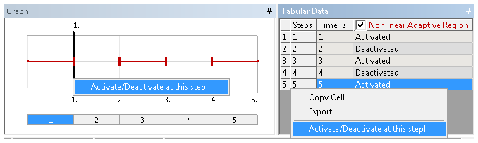
Note: You may wish to review the Activation/Deactivation of Loads topic in the Step Controls section of the Help. The Nonlinear Adaptive Region condition is displayed in the graph for the Analysis Settings object.
Details View Properties
The selections available in the Details view are described below.
| Category | Properties/Options/Description |
|---|---|
| Scope |
Scoping Method, options include:
You may wish to review the Mechanical APDL References and Notes at the bottom of the page for specific command execution information regarding these selections. |
| Definition |
Criterion: Options included , , or .
All the following common criteria properties are available for all Criterion property options as well as 2D analyses:
Suppressed: Include ( - default) or exclude () the condition. |

Initial Mesh Load Specifications
You can apply the following boundary conditions directly to the initial mesh generated for each load step rather than on the newly generated mesh only by setting the object's Apply To Initial Mesh property to .
For more information, see the Initial-Mesh Loading and Constraint section in the Nonlinear Adaptivity Analysis Guide of the Mechanical APDL documentation.
View Changed Mesh Results
Following the solution process, to determine if the mesh was changed:
Select the Solution object or a Result object, the Tabular Data window displays the substeps with a changed mesh (Changed Mesh column = ).
Select the Solution Information object and set the Solution Output property to . A chart displays. Remesh Points are shown by solid orange vertical lines.
Create a User Defined Result (using the PNUMELEM Expression) to view the new elements that have relatively larger element identities than the original element identities. You can duplicate this result and specify a ( property) for a result prior to a remesh and one at a remesh point, and using the Viewports feature, directly compare the (before and after) elements in the graphics window.
Mechanical APDL References and Notes
The following Mechanical APDL commands, element types, and considerations are applicable for this condition.
The Nonlinear Adaptive Region is applied with the NLADAPTIVE command.
When the Scoping property is defined as , the Nonlinear Adaptive Region condition uses the CM command to create the Nonlinear Adaptive Region component.
When the Scoping property is defined as a , the Nonlinear Adaptive Region condition uses the CMBLOCK command to create the Nonlinear Adaptive Region component.
The CMSEL,ALL command and the ESEL,ALL command are issued at beginning of the NLADAPTIVE command.
During a Structural Analysis, the Nonlinear Adaptive Region is applied using the PLANE182 (2-D Low Order), PLANE183 (2-D High Order), SOLID285 (3-D Linear Tetrahedral), and SOLID187 (3-D Quadratic Tetrahedral) element types.
When a Nonlinear Adaptive Region is scoped to a body/element, the associated part is meshed with SOLID285 element type if they are linear tetrahedral or SOLID187 element type if they are quadratic tetrahedral.
When a Nonlinear Adaptive Region is deactivated for certain steps, the NLADAPTIVE command is set to be OFF in the corresponding load steps. Relatively, an activated Nonlinear Adaptive Region sets the NLADAPTIVE command to be ON.
When a Nonlinear Adaptive Region is applied, the ETCONTROL ,SET command is not issued.
Note: For additional guidance about how to best use this feature, see the Mesh Nonlinear Adaptivity Hints and Recommendations section in the Mechanical APDL Advanced Analysis Guide.
Nonlinear Adaptive Region Solving Limitations
The purpose of nonlinear adaptive region is to repair a distorted mesh in order to overcome convergence problems caused by the distortion. It is effective only when the mesh distortion is caused by a large, nonuniform deformation. Nonlinear adaptive region cannot help if divergence occurs for any other reason such as unstable material, unstable structures, or numerical instabilities.
Unstable Material
Most nonlinear material models, especially those employing hyperelastic materials, have their own applicable ranges. When a deformation is too large or a stress state exceeds the applicable range, the material may become unstable. The instability can manifest itself as a mesh distortion, but nonlinear adaptive region cannot help in such cases. While it is sometimes difficult to determine when material is unstable, you can check the strain values, stress states, and convergence patterns. A sudden convergence difficulty could mean that material is no longer stable. The program also issues a warning at the beginning of the solution indicating when hyperelastic material could be unstable, although such a warning is very preliminary and applies only to cases involving simple stress states.
Unstable Structures
For some geometries and loads, a deformation may cause a "snap-through," or local buckling. Such behavior can also manifest itself as a mesh distortion, but one that nonlinear adaptive region cannot repair. The effect is usually easy to detect by closely checking the deformed region or the load-versus- time (displacement) curve.
Numerical Instabilities
A condition of numerical instability can occur when a problem is nearly overconstrained. The constraints can include kinematic constraints such as applied displacements, couplings, and constraint equations, and volumetric constraints introduced by fully incompressible material in mixed u-P elements. In many cases, numerical instability is apparent even in the early stages of an analysis.