


You can find information about Boundary Conditions in Apply Loads and Supports. For an LS-DYNA system, Remote Displacement is available in addition to the boundary conditions discussed there.
The Conditions 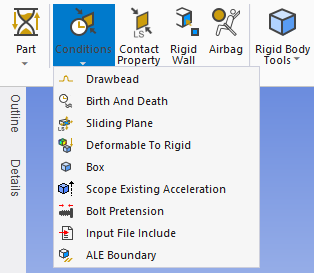 ,
Contact Property
,
Contact Property ![]() , and Rigid Wall
, and Rigid Wall
![]() constraints are
available on the LSDYNA Pre tab. The following boundary conditions are also available:
constraints are
available on the LSDYNA Pre tab. The following boundary conditions are also available:
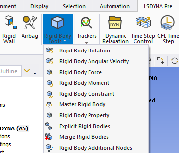
Use the Rigid Body Tools to specify the behavior of the rigid bodies in your model.
Rigid Body Rotation
 -
specify the rotation of a rigid body(ies).
-
specify the rotation of a rigid body(ies).Rigid Body Angular Velocity
 -
specify the angular velocity of a rigid body(ies).
-
specify the angular velocity of a rigid body(ies).Rigid Body Force
 - apply a
force to the center of mass of a rigid body(ies).
- apply a
force to the center of mass of a rigid body(ies).Rigid Body Moment
 - apply a
moment to a rigid body(ies).
- apply a
moment to a rigid body(ies).Rigid Body Constraint
 -
constrain the motion of a rigid bod(dies).
-
constrain the motion of a rigid bod(dies). Master Rigid Body
 - link
multiple rigid bodies together. The master rigid body leads the movement of the other
linked bodies.
- link
multiple rigid bodies together. The master rigid body leads the movement of the other
linked bodies. Rigid Body Property
 - set
the mass, center of mass, and mass moment of inertia of a rigid body.
- set
the mass, center of mass, and mass moment of inertia of a rigid body. Explicit Rigid Bodies
 - identify
body(ies) that are rigid in an LS-Dyna Explicit analysis and flexible in other types of
analyses.
- identify
body(ies) that are rigid in an LS-Dyna Explicit analysis and flexible in other types of
analyses.Merge Rigid Bodies
 - merge
multiple rigid bodies together into a single rigid body.
- merge
multiple rigid bodies together into a single rigid body.Rigid Body Additional Nodes
 - add
additional nodes from a flexible body to an existing rigid body.
- add
additional nodes from a flexible body to an existing rigid body.
Use the Rigid Body Rotation tool ![]() to specify the
rotation of a rigid body (or bodies) in radians. This command rotates the selected rigid
body(ies) around the x-axis, y-axis, or z-axis of the global coordinate system according
to the rotation curve you enter.
to specify the
rotation of a rigid body (or bodies) in radians. This command rotates the selected rigid
body(ies) around the x-axis, y-axis, or z-axis of the global coordinate system according
to the rotation curve you enter.
Select the rigid body(ies) to be rotated, specify the axis of rotation, and define the times and magnitudes of the rotation curve in a table. For more complex rotations, break the rotation down into its x-, y-, and z-components and define separate rigid body rotation objects for rotation around each axis.
During the solution, the LS-DYNA solver applies a force to rotate the rigid body(ies) according to the rigid body rotation direction(s) and curve(s) you entered. It starts each rotation curve at the birth time and stops it at the death time.
Details of "Rigid Body Rotation"
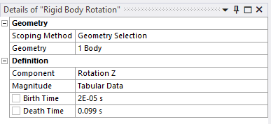
Specify the input parameters for the Rigid Body Rotation tool:
| Field | Description |
|---|---|
| Scoping Method | Choose the method for selecting one or more rigid bodies. Only select objects
that were defined as rigid bodies.
|
| Geometry | Displays the number of selected rigid bodies. |
| Component | Choose the axis of rotation for the selected rigid body(ies): Rotation X, Rotation Y, or Rotation Z. Rotation can be specified independently for each axis. |
| Magnitude | Enter the time steps and magnitude of the rotation of the selected rigid bodiy(ies) (that is, the rotation curve). See Tabular Data for Rigid Body Rotation (below). |
| Birth Time | Enter the time when the LS-DYNA solver begins executing the rotation curve
defined under Tabular Data for Rigid Body
Rotation. The boundary condition becomes
active at that time and is used in the solution. The Birth Time is set independently of the rotation start time defined under Tabular Data. |
| Death Time | Enter the time when the LS-DYNA solver stops executing the rotation curve
defined under Tabular Data for Rigid Body
Rotation. The boundary condition
becomes inactive and is no longer used in the solution. The Death Time is set independently of the rotation end time defined under Tabular Data. |
Tabular Data for Rigid Body Rotation
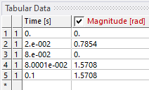
Use this table to enter a rotation curve that specifies how the selected rigid body(ies) rotate. At each step in the curve, enter the time and magnitude of rotation.
| Column | Description |
|---|---|
| 1, 2, 3 … * | The first column shows the time step of the rotation curve. Each time step is
numbered in order of its execution during the solution. Enter a new time and magnitude into the * field. See Adding Time Steps to the Rigid Body Rotation Curve (below). |
| 1, N/A | The second column shows whether the time step occurs (and is used) during the solution
|
| Time [s] | The time in seconds at which rotation occurs. The first time step defaults to zero. The last time step defaults to the end of the solution time. |
| Magnitude [rad] | The magnitude of rotation in radians. |
Adding Time Steps to the Rigid Body Rotation Curve
You can manually enter a Time and Magnitude of rotation in the row marked with *. Alternatively, you can copy and paste pairs of time and magnitude values from a spreadsheet into that row.
The system adds these values to the table according to their Time value.
If you enter a Time between the start time (time step 1) and the end time (the last numbered time step in the table), the system adds the time step to the table in order of its time value.
If you enter a Time without a corresponding Magnitude, the system automatically assigns a rotation value that is interpolated between the two surrounding time steps. You can then change the magnitude of rotation to the desired value.
If you enter a time value after the end time, the system adds it to the table as an N/A row. It is not used during the solution.
Graph of Rigid Body Rotation Curve
The Graph panel plots the rotation curve that you defined under Tabular Data. Click the check box next to Magnitude [rad] in the Tabular Data table to toggle the display of this curve.
Use the Rigid Body Angular Velocity tool ![]() to set the angular
velocity of the rigid body in radians per second . This command applies an angular
velocity to the selected rigid body(ies) around the x-axis, y-axis, or z-axis of the
global coordinate system according to the angular velocity curve you specify.
to set the angular
velocity of the rigid body in radians per second . This command applies an angular
velocity to the selected rigid body(ies) around the x-axis, y-axis, or z-axis of the
global coordinate system according to the angular velocity curve you specify.
Select the rigid body(ies) to which an angular velocity is applied, specify the axis of rotation, and define the angular velocity curve (that is, the times and magnitudes of angular velocity) in a table. For more complex rotation patterns, break the angular velocity down into its x-, y-, and z-components and define separate rigid body angular velocity objects for the angular velocity around each axis.
During the solution, the LS-DYNA solver applies a force to the rigid body to rotate it according to the angular velocity direction(s) and curve(s) you entered. It starts to execute each angular velocity curve at the birth time and stops it at the death time.
Details of "Rigid Body Angular Velocity"
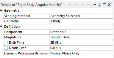
Specify the input parameters for the Rigid Body Angular Velocity tool:
| Field | Description |
|---|---|
| Scoping Method | Choose the method for selecting one or more rigid bodies. See the discussion of Scoping Method under Details of "Rigid Body Rotation". |
| Geometry | Displays the number of selected rigid bodies. |
| Component | Select the axis of rotation for the selected rigid body(ies). See the discussion of Component under Details of "Rigid Body Rotation". |
| Magnitude | Enter the time steps and magnitude of the angular velocity of the selected rigid body(ies) (that is, the angular velocity curve). See Tabular Data for Rigid Body Angular Velocity (below). |
| Birth Time | Enter the time when the LS-DYNA solver begins executing the angular velocity
curve that is defined under Tabular Data for
Rigid Body Angular Velocity . The boundary
condition becomes active at that time and is used in the solution. The Birth Time is set independently of the angular velocity start time defined under Tabular Data. |
| Death Time | Enter the time that the solver stops executing the rigid body angular
velocity curve that is defined under Tabular Data for
Rigid Body Angular Velocity . The boundary
condition becomes inactive and is no longer used in the solution. The Death Time is set independently of the angular velocity end time defined under Tabular Data. |
| Dynamic Relaxation Behavior | Dynamic relaxation sets the preloading for explicit dynamics solutions in
LS-DYNA. Select one of the following:
See Dynamic Relaxation for more information. |
Tabular Data for Rigid Body Angular Velocity
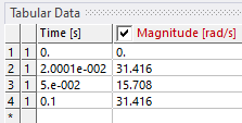
Use this table to enter the angular velocity curve, which specifies how the system applies angular velocities to the selected rigid body(ies). Enter the Time in seconds and the Magnitude of the angular velocity in radians per second. See Tabular Data for Rigid Body Rotation for more information.
Graph of Rigid Body Angular Velocity Curve
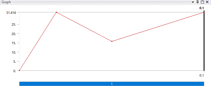
The Graph panel plots the angular velocity curve that you defined under Tabular Data. Click the check box next to Magnitude [rad/s] in the Tabular Data table to toggle the display of this curve.
Use the Rigid Body Force tool ![]() to apply a force to a
rigid body. This command applies a force in the x, y, or z direction to the center of mass
of the selected rigid body(ies), according to the force curve you specify.
to apply a force to a
rigid body. This command applies a force in the x, y, or z direction to the center of mass
of the selected rigid body(ies), according to the force curve you specify.
Select the rigid body(ies) to which a force is applied, specify the direction, and define the force curve (that is, the times and magnitudes at which force is applied) in a table. You can decompose a force vector into its x, y, and z components and define separate rigid body force objects for each component.
During the solution, the LS-DYNA solver applies a force to the rigid body according to the force direction(s) and curve(s) you entered. The solver starts to execute each force curve at the start time under Tabular Data and stops it at the end time.
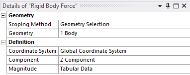
Details of "Rigid Body Force"
| Field | Description |
|---|---|
| Scoping Method | Choose the method for selecting one or more rigid bodies. See the discussion of Scoping Method under Details of "Rigid Body Rotation". |
| Geometry | Displays the number of selected bodies. |
| Coordinate System | Specifies the coordinate system (defaults to Global Coordinate System) |
| Component | Specify which component of the force vector you are defining (X Component, Y Component, or Z Component). |
| Magnitude | Enter the time steps and magnitude of the force that is applied to the selected rigid body(ies) (that is, the force curve). See Tabular Data for Rigid Body Force (below). |
Tabular Data for Rigid Body Force
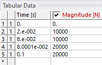
Use this table to enter the force curve, which specifies how the system applies a force to the selected rigid body(ies). Enter the Time in seconds and the Magnitude of the force in Newtons. See Tabular Data for Rigid Body Rotation for more information.
Graph of Rigid Body Force Curve
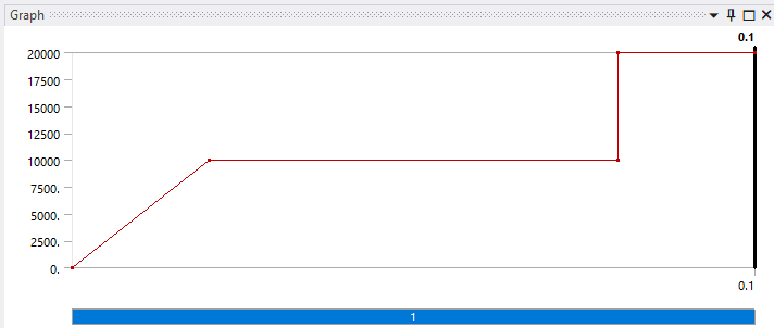
The Graph panel plots the force curve that you defined under Tabular Data. Click the check box next to Magnitude [N] in the Tabular Data table to toggle the display of this curve.
Use the Rigid Body Moment tool ![]() to apply a moment to a
rigid body. This command applies a moment in the x, y, or z direction to the selected
rigid body(ies), according to the moment curve you specify.
to apply a moment to a
rigid body. This command applies a moment in the x, y, or z direction to the selected
rigid body(ies), according to the moment curve you specify.
Select the rigid body(ies) to which a moment is applied, specify the direction, and define the moment curve (that is, the times and magnitudes at which a moment is applied) in a table. You can decompose a moment vector into its x, y, and z components and define separate rigid body moment objects for each component.
During the solution, the LS-DYNA solver applies a moment to the rigid body according to the direction(s) and curve(s) you entered. The solver starts to execute each moment curve at the start time under Tabular Data and stops it at the end time.
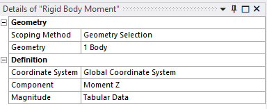
Details of "Rigid Body Moment"
| Field | Description |
|---|---|
| Scoping Method | Choose the method for selecting one or more rigid bodies. See the discussion of Scoping Method under Details of "Rigid Body Rotation". |
| Geometry | Lists the number of selected bodies. |
| Coordinate System | Specifies the coordinate system (defaults to Global Coordinate System) |
| Component | Specify which component of the moment vector you are defining (Moment X , Moment Y , or Moment Z ). |
| Magnitude | Enter the time steps and magnitude of the moment that is applied to the selected rigid body(ies) (that is, the force curve). See Tabular Data for Rigid Body Moment (below). |
Tabular Data for Rigid Body Moment
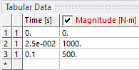
Use this table to enter the moment curve, which specifies how the system applies a moment to the selected rigid body(ies). Enter the Time in seconds and the Magnitude of the force in Newton-meters. See Tabular Data for Rigid Body Rotation for more information.
Graph of Rigid Body Moment Curve
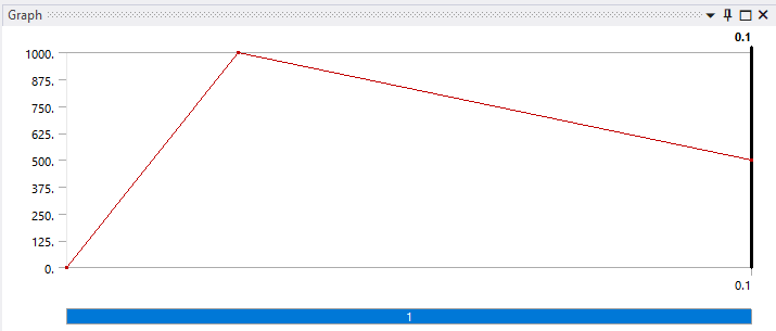
The Graph panel plots the moment curve that you defined under Tabular Data. Click the check box next to Magnitude [N·m] in the Tabular Data table to toggle the display of this curve.
Use the Rigid Body Constraint tool ![]() to constrain the
motion of a rigid body. This tool allows you to specify the degrees of freedom for the
selected rigid body(ies). You can constrain their movement in the x, y, or z direction and
their rotation around the global x, y, or z axis.
to constrain the
motion of a rigid body. This tool allows you to specify the degrees of freedom for the
selected rigid body(ies). You can constrain their movement in the x, y, or z direction and
their rotation around the global x, y, or z axis.
Details of "Rigid Body Constraint"
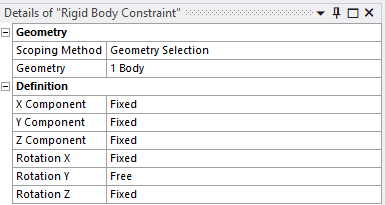
| Field | Description |
|---|---|
| Scoping Method | Choose the method for selecting one or more rigid bodies. See the discussion of Scoping Method under Details of "Rigid Body Rotation". |
| Geometry | Lists the number of selected bodies. |
| X Component Y Component Z Component | Choose whether the rigid body's movement in the x, y or z direction is Fixed (cannot move in that direction) or Free (no restriction on movement in that direction). |
| Rotation X Rotation Y Rotation Z | Choose whether the rigid body's rotation around the x, y or z axis is Fixed (cannot rotate around that axis) or Free (no restriction on rotation around that axis). |
Use the Master Rigid Body tool ![]() to link two or more
rigid bodies together. The rigid bodies must be connected by a mesh.
to link two or more
rigid bodies together. The rigid bodies must be connected by a mesh.
In the Mechanical workbench, the components of a larger body can be grouped together. When this group contains rigid bodies, the LS-DYNA solver merges the rigid bodies and computes a single solution for them. By using the Master Rigid Body tool, you can pick which rigid body in this group is assigned boundary conditions (the master rigid body). The solver applies any rigid body boundary conditions to the master rigid body you select. The master rigid body leads the movement of the rigid bodies that are connected to it by a mesh. The connected rigid bodies are constrained to move with the master rigid body.
Use the Merge Rigid Bodies tool to combine rigid bodies that are not connected by a mesh.
Details of "Master Rigid Body"
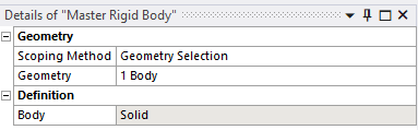
Select the master rigid body.
| Field | Description |
|---|---|
| Scoping Method | Specify the method for selecting a body. See the discussion of Scoping Method under Details of "Rigid Body Rotation". |
| Geometry | Lists the number of selected bodies. |
| Body | The type of body selected as the master rigid body. |
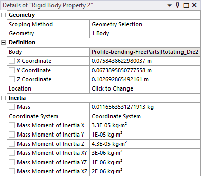
Use the Rigid Body Property tool ![]() to set the following
rigid body properties:
to set the following
rigid body properties:
| Field | Description |
|---|---|
| Scoping Method | Specify the method for selecting a rigid body. Only select objects that were
defined as rigid bodies.
|
| Body, Coordinates | After the Geometry is scoped to the Rigid Body Property object, the name of the body is displayed and the coordinates of the center of mass are transferred from the scoped body to the Coordinates fields. |
| Location | Use this field to change the location of the center of mass of the body. |
| Mass, Moments of Inertia | The Mass and Moments of Inertia are transferred from the scoped body to these fields. |
| Coordinate System | Select the coordinate system in which you want to display the center of mass. |
The Rigid Body Property tool allows you to set the mass, center of mass, and mass moment of inertia of a rigid body. When scoping a body to the geometry, the name of the Body is displayed, and the properties X,Y,Z coordinates, mass, and moments of inertia are filled accordingly from the values in the Geometry object. You can change the center of mass by scoping a geometric entity to the Location. When scoping multiple geometric entities, the equivalent center of mass is computed. The equivalent center of mass is the weighted mean of the center of gravity times the mass of all geometric entities. If you change the mass, the mass moments of inertia will be multiplied by the ratio between the new entered mass by the already scoped bodies mass.
Use the Explicit Rigid Bodies tool ![]() to identify body(ies) that are
treated as being rigid in an LS-DYNA Explicit analysis and flexible in other types of
analyses.
to identify body(ies) that are
treated as being rigid in an LS-DYNA Explicit analysis and flexible in other types of
analyses.
Details of "Explicit Rigid Bodies"
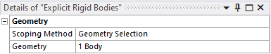
Select the body(ies) that are treated as rigid during an Explicit analysis.
| Field | Description |
|---|---|
| Scoping Method | Specify the method for selecting a body. See the discussion of Scoping Method under Details of "Rigid Body Rotation". |
| Geometry | Lists the number of selected bodies. |
Use the Merge Rigid Bodies tool ![]() to combine multiple rigid
bodies together into a single rigid body. The rigid bodies do not have to be adjacent.
to combine multiple rigid
bodies together into a single rigid body. The rigid bodies do not have to be adjacent.
Ordinarily, the LS-DYNA solver considers each rigid body separately. By using the Merge Rigid Body tool, you can combine the selected rigid bodies into a single body. All rigid body boundary conditions are applied to the master rigid body. The slave rigid bodies are constrained to move with the master rigid body.
Details of "Merge Rigid Bodies"
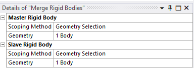
Select the Master Rigid Body and at least one Slave Rigid Body.
| Field | Description |
|---|---|
| Scoping Method | Specify the method for selecting a rigid body. See the discussion of Scoping Method under Details of "Rigid Body Rotation". |
| Geometry | Lists the number of selected bodies. |
Use the Rigid Body Additional Nodes tool ![]() to create additional
nodes in the mesh between adjacent rigid and flexile bodies. This adds rigid nodes to the
flexible body, which creates a better connection and prevents deformation between the
rigid and flexible bodies.
to create additional
nodes in the mesh between adjacent rigid and flexile bodies. This adds rigid nodes to the
flexible body, which creates a better connection and prevents deformation between the
rigid and flexible bodies.
Details of "Rigid Body Additional Nodes"
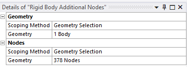
Under Geometry, select the desired rigid body. Under Nodes, select the desired entities (non-body geometry scopings or nodes) to be added to the selected rigid body. The system adds nodes to the mesh for the selected entities.
| Field | Description |
|---|---|
| Scoping Method | Specify the method for selecting a body. See the discussion of Scoping Method under Details of "Rigid Body Rotation". |
| Geometry | Geometry - Lists the number of selected
bodies. Nodes - Lists the number of nodes that are added. |
The Airbag object provides a way of defining thermodynamic behavior of the gas flow into the airbag as well as a reference configuration for the fully inflated bag.
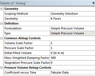
Simple Pressure Volume
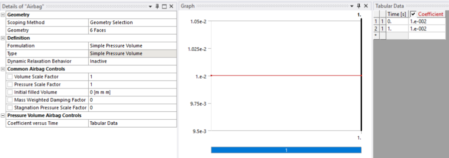
When Formulation is set to Simple Pressure Volume:
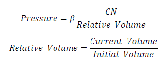
The pressure is a function of the ratio of current volume to the initial volume.
This simple model can be used when an initial pressure is given.
No leakage, no temperature change, and no input mass flow are assumed.
A typical application is the modeling of air in automobile tires.
Pressure Volume Airbag controls: Coefficient versus Time (CN) can be defined in a table. β is a scale factor for the curve defining the coefficient versus time (CN), with a default value of 1.
Simple Airbag Model
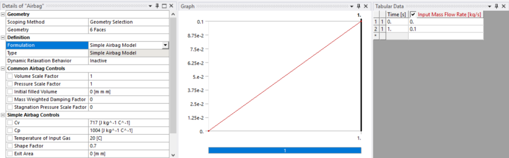
The volume pressure relationships is defined by the Simple Airbag Model for control volumes.
The gamma law equation of state used to determine the pressure in the airbag:
p = (γ-1)ρe
where p is the pressure, ρ is the density, e is the specific internal energy of the gas, and γ is the ratio of the specific heats:
γ = cp/cv
Input Mass Flow Rate can be defined in a table.
Load Curve Airbag Model
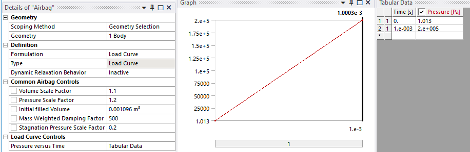
You can supply a tabular load curve to define the pressure as a function of time.
Advanced users can insert additional LS-DYNA keywords by using the
Input File Include constraint to specify the name of a file
that contains LS-DYNA keywords. An include file *INCLUDE
Filename1 keyword card will be generated pointing to the file you
specify.
Included files can contain any valid LS-DYNA keyword cards. Using include files eliminates the need for you to edit the .k input file each time the file is created by LS-DYNA if you have other keywords you want to use. Note that the included file can contain other include file statements, providing a fairly general capability for easily adding predefined inputs.
You can also insert additional LS-DYNA keywords by using the Keyword Snippet (LS-DYNA) constraint. Create a Keyword Snippet (LS-DYNA) object by inserting a Commands object from the context menu or Enviroment tab on the ribbon.
Note: When inserted under Connections, the Keyword Snippet (LS-DYNA) object allows you to use contact types not supported by the LS-DYNA system. When inserted under the Environment object, it allows you to use any LS-DYNA keywords.
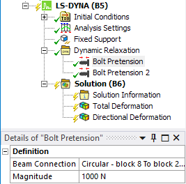
This boundary condition applies a pretension load to a beam connection, typically to model a bolt under pretension.
Analysis Types
Bolt Pretension is specific to LS-DYNA and is not compatible with the Bolt Pretension feature of the Mechanical Application.
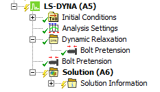
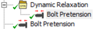
The Bolt Pretension can be either used during dynamic relaxation or during the explicit phase of the calculation.
A Bolt Pretension can be applied to either a Beam Connection or a Solid Body.
Boundary Condition Application
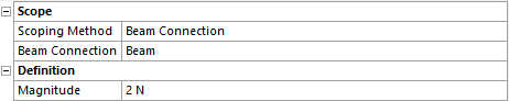
To apply a Bolt Pretension to a Beam Connection:
Right-click the Environment tree object or an active Dynamic Relaxation Object and select > .
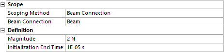
Set the Scoping Method to Beam Connection and then select the Beam Connection.
Specify the Magnitude of the loading.
If the bolt pretension is used during the explicit phase, you need additionally an Initialization End Time to specify the termination of the loading.
To apply a Bolt Pretension to a Solid Body:
Right-click the Environment tree object or an active Dynamic Relaxation Object and select > .
Set the Scoping Method to Geometry Selection or Named Selection and then select the Solid Body
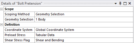
Specify a Coordinate System to define the cutting plane. The cutting plane is centered on the origin of the selected Coordinate System and aligned with the X-Y plane.
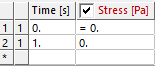
Define the pre-load stress as a function of time using the Tabular Data field, and define the type of Shear Stresses acting on the body with the Shear Stress Flag.
Note:
The Bolt Pretension Load is not supported for a Full Restart.
When a Bolt Pretension within the Dynamic Relaxation Folder and a Bolt Pretension under the LS-DYNA Transient Analysis are defined for the same Beam connection, only the last one defined is used in the analysis.
The dynamic relaxation feature (available by clicking ![]() on the LSDYNA Pre
tab, or by right-clicking the LS-DYNA system and selecting Dynamic Relaxing from
the Insert menu) provides preloading for explicit dynamics solutions in LS-DYNA.
True dynamic relaxation (Relaxation Type: Explicit) allows an
explicit solver to conduct a static analysis by increasing the damping until the
kinetic energy drops to zero.
on the LSDYNA Pre
tab, or by right-clicking the LS-DYNA system and selecting Dynamic Relaxing from
the Insert menu) provides preloading for explicit dynamics solutions in LS-DYNA.
True dynamic relaxation (Relaxation Type: Explicit) allows an
explicit solver to conduct a static analysis by increasing the damping until the
kinetic energy drops to zero.
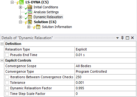
The damping works by scaling nodal velocities by the Dynamic Relaxation Factor each time step until the ratio of current distortional kinetic energy to peak distortional kinetic energy (the convergence factor) falls below the convergence tolerance (Tolerance).
By default, the convergence is checked on the whole model. It can be restricted to a set of bodies by setting the Convergence Scope to Geometry Selection.
When the Ansys Implicit solver is used to provide the preload (Relaxation Type: Explicit After Ansys Solution), a slightly different approach is taken in that the stress initialization is based on a prescribed geometry (in other words, the nodal displacement results from the Implicit solution). In this case, the explicit solver only uses 101 time steps to apply the preload. In the former case, the solver will check the kinetic energy every 250 cycles (by default) until the kinetic energy from the applied preload is dissipated.
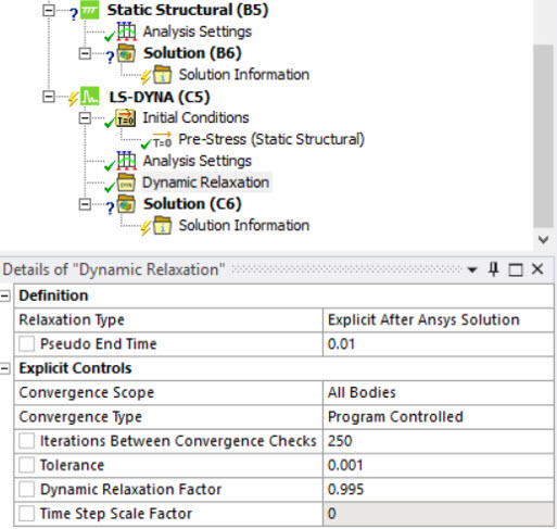
If the Convergence Type is set to Termination occurs at Pseudo End Time instead of Program Controlled, the termination of the dynamic relaxation occurs at the pseudo end time.
The Time Step Scale Factor enables you to scale the computed time step during dynamic relaxation.
Alternatively, the LS-DYNA Implicit solver can be used to conduct a dynamic analysis to calculate the preloading.
An initial time step must be provided to start the nonlinear implicit transient analysis. The convergence of this Newton-Raphson analysis is controlled by the Line Search convergence tolerance and a Displacement Convergence tolerance.
LS-DYNA supports all these methods, which occur in pseudo time before the transient portion of the analysis begins at time zero.
Preloading
Preloading works by specifying that a given load will be active during the dynamic relaxation, when the relaxation type is set to Explicit or Implicit.
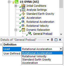
Currently, Acceleration, Standard Earth Gravity, Rotational Acceleration and Rotational Velocity can be specified as a Load in the General Preload object for dynamic relaxation.
Other Loads and Supports can be applied during dynamic relaxation through the use of an option on the Load/Support.
Preloading using General Preload
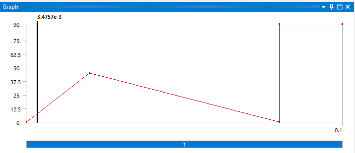
When the User Defined field is set to No, the load used during the dynamic relaxation phase is represented by the following curve:
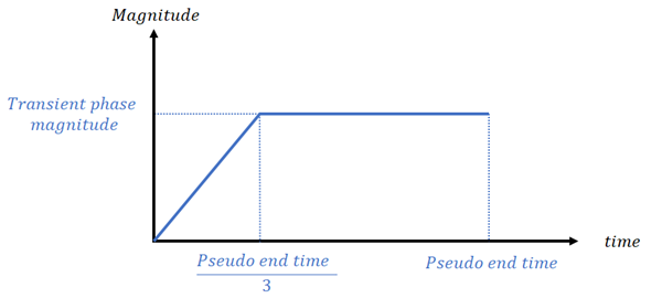
For the boundary condition undergoing dynamic relaxation, an additional curve (*DEFINE_CURVE) is written defining the load magnitude during the dynamic relaxation phase. The standard curve shown above is applied only during the dynamic relaxation phase (preloading) as SIDR=1 in the *DEFINE_CURVE.
When the User Defined field is set to Yes, you can enter a customized curve for the dynamic relaxation phase by filling a data table.
When the load is user defined, the card *DEFINE_CURVE with the SIDR parameter set to 1 will be written to the input file. This curve is then used by the card representing the boundary condition to which the dynamic relaxation is applied.
Note: Unlike other Dynamic Relaxation loads compatible with the General Preload object, both Rotational Velocity and Rotational Acceleration do not use any directional General Preload Scale Factor. This is related to limitations from the LS-DYNA card *LOAD_BODY_GENERALIZED that is used. It is still possible to apply these loads in specific directions, through the definition of the Coordinate System property in the Rotational Velocity or Rotational Acceleration objects themselves. Be mindful that the same preload curve will be applied to any loaded direction in these objects.
Preloading using a Load/Support Option
Dynamic relaxation can be defined in a simpler way for several loads (including Pressure, Force, Nodal Force, and Rigid Body Angular Velocity), and Supports that are defined so that they are not fixed. For these boundary conditions, the Dynamic Relaxation Behavior field is added to their Details panel. This field has three options:
Normal Phase Only - The boundary condition is applied during the explicit solution only
Dynamic Relaxation Only - The boundary condition is applied during preloading only
Both - The boundary condition is applied in both phases
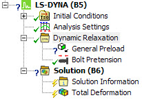
Preloading using Bolt Pretension
LS-DYNA also enables preloading of Beam Connections through the Bolt Pretension.
A Box is an object that can be used to define a behavior for a set of nodes. For instance, it can be used to specify that SPH computations occur for particles inside the box.
To insert a box in an LS-DYNA analysis, right-click the system and select > .
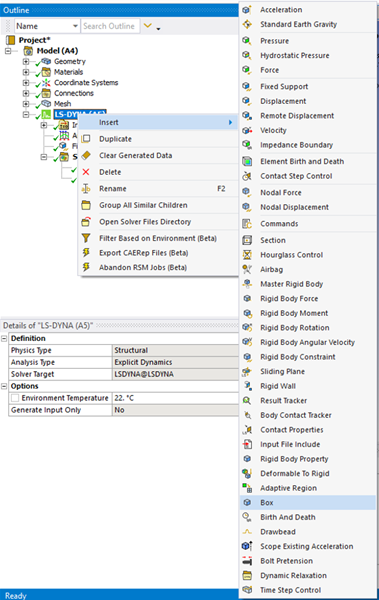
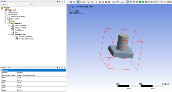
Two types of boxes exist: Standard and SPH. The Standard box is a stationary box. At this time, its function is to limit the SPH or SPG computation to particles that are within the box at the beginning of the simulation.
For the Standard box, the input parameters are:
The boundary of the box defined by the coordinates of two diagonally opposite corner points: Xmin, Xmax, Ymin, Ymax, Zmin, Zmax.
The Coordinate System that defines the orientation of the box. You can define a customized coordinate system (new origin and new orientation) then select that coordinate system to assign it to the box.
The SPH box is a standard box that can move over time and is used only for SPH calculations. The SPH Box Motion Controls section in the Details panel allows you to specify the motion Type as a Displacement or Velocity. The direction of the box motion is defined by the Coordinate System and the Component. You can define time-dependent velocity or displacement for the box motion by entering tabular data.
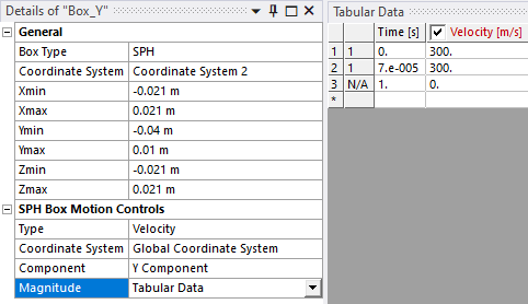
Note: For SPH analyses, the box must include the contact surface region between the particles and the Lagrangian region in order to properly determine the mechanical behavior.
You can define any number of Standard and SPH boxes in an analysis. In conjunction with the Use Box analysis setting, the following rules govern the solver's use of the boxes defined in the analysis.
- If Use Box is set to No
Any Standard boxes defined in the analysis will not be used. However, if you have an unsuppressed SPH box, then the calculation will occur with respect to the SPH box. If you have multiple unsuppressed SPH boxes, then the solver will consider the first defined SPH box.
- If Use Box is set to Yes
If you only have Standard boxes defined, you can choose a Standard box from the Box Name drop down.
If you only have SPH boxes defined, you don't need to set the Box Name because the first unsupressed defined SPH box will be used. An information message will be output indicating the Box that is used.
If you have both Standard and SPH boxes defined, if you choose a Standard box from the Box Name drop-down, the solver will ignore that box and will use the first unsuppressed SPH box that is defined. When an SPH box is used, an information message will pop up to indicate the Box used by the solver.
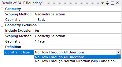
The ALE Boundary object can be applied to bodies with Reference Frame set to S-ALE Domain, or contained in a section definition with an ALE element formulation. When an ALE Boundary object is included in the analysis, an *ALE_ESSENTIAL_BOUNDARY card is written. Two constraint types are available, which will be applied to the external faces of the main geometry selection except for any faces defined in the exclusion scoping.
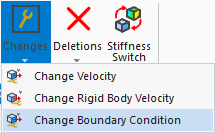
The Change Boundary Condition load can be inserted in an LS-DYNA Small Restart analysis and allows you to change the definition of an existing *DEFINE_CURVE keyword in the input.k file. The Change Boundary Condition load can be found on the LSDYNA Small Restart tab of the ribbon.
The *DEFINE_CURVE keyword is written to the input file when tabular data is provided for a load. The Change Boundary Condition object is needed because in an LS-DYNA analysis, the end time of the tabular data defined in the analysis cannot exceed the end time of the analysis itself. For example, a Displacement Component is defined by a Tabular Data in an initial LS-DYNA analysis and you want to continue with a Small Restart. You cannot change the values of the Displacement Component for the Restart analysis (the object is unavailable in the Small Restart). The Change Boundary Condition object gives you this ability.
The load will redefine a *DEFINE_CURVE that already exists in the initial (or one of the previous) analyses. The tabular data you enter must correspond to the size of the table in the existing *DEFINE_CURVE. The *DEFINE_CURVE to be modified might have been generated by the Tabular Data defining one of the degrees of freedom of a boundary condition (currently, only Displacement and Remote Displacement are supported).
When you insert a Change Boundary Condition object, the Location Method will be set to Boundary Condition.
You will see the following fields in the Details panel. Once you choose a Boundary Condition from the drop-down list, fields will appear corresponding to the components using tabular data in that boundary condition.
| Field | Input Values | Description |
|---|---|---|
| Location Method | Boundary Condition | Specifies that the tabular data to be redefined is in a boundary condition |
| Boundary Condition | Drop-down with available boundary conditions | Specifies which boundary condition needs to have tabular data redefined |
| Component | X/Y/Z Component | Specifies which degree of freedom will have the tabular data in its *DEFINE_CURVE redefined |
| Curve | Tabular Data | Allows redefinition of the data in the *DEFINE_CURVE associated with the component |
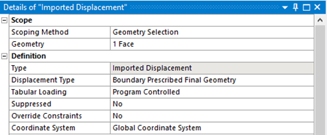
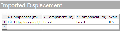
The External Data system allows you to import external loads into an LS-DYNA analysis. Currently, the loads supported for LS-DYNA analyses are Imported Pressure and Imported Displacement.
When an Imported Displacement is added to an LS-DYNA analysis, the keyword written to the input file is determined by the Displacement Type field. The two keyword options are Boundary Prescribed Final Geometry and Initial Foam Reference Geometry.
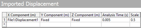
When selecting the displacement for each component in the Data View worksheet, the Free option available for other types of analyses is not shown as it is not applicable when using these LS-DYNA keywords.
When the Displacement Type is set to Initial Foam Reference Geometry the Tabular Loading field is hidden. The rate at which the displacement is applied is determined by the solver in this case.
The Displacement Type Initial Foam Reference Geometry is only applicable to a subset of materials. Refer to the description of *Initial_Foam_Reference_Geometry in LS-DYNA Keyword User's Manual Volume I for a list of the supported material types.
Note: When the Imported Displacement is scoped to a body with a supported material, the reference geometry flag on the material card is automatically set. If the material is defined using a command snippet, the reference geometry flag is not automatically set and the value given in the snippet is written directly to the input file.