


The general guidelines for setting up an explicit dynamics analysis can be found in Explicit Dynamics Workflow. LS-DYNA related information is included in that chapter. The use of the LS-DYNA system is described in this section.
You can find information about Materials in Define Engineering Data.
Note:
The Material Assignment folder is not supported by LS-DYNA.
In Engineering Data, temperatures defined in the Material Field Variable section are not used by the LS-DYNA analysis system. In general coefficients that are temperature dependent are not taken into account. Only the first value in the table is used for these coefficients, and you can only have one reference temperature even if multiple materials are used in the model.
You can find information about Geometry in Attach Geometry.
Note: LS-DYNA cross sections are not fully compatible with cross sections available in Design Modeler. When using a LS-DYNA system the Z, Hat ,and Channel cross sections are exported with the following limitations.
For the Z cross section, the LS-DYNA type 6 is used. It imposes the following restrictions:
W1 = W2 (W2 is assumed equal to W1)
t1 = t2 (t1 is assumed equal to t2)
For the Hats cross section, the LS-DYNA type 21 is used. It imposes the following restrictions:
W1 = W2 (W2 is assumed equal to W1)
t1 = t2 = t3 = t4 = t5
For the Channel cross section, the LS-DYNA type 2 is used. It imposes the following restrictions:
W1 = W2 (W2 is assumed equal to W1)
t1 = t2 (all the thicknesses are assumed identical)
You can find information about Part Behavior in Define Part Behavior.
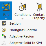
Add the objects under Part from the LSDYNA Pre tab to specify Section properties such as element formulations, and specify different Hourglass Control objects for each part. You can also add an Adaptive Region or an Adaptive Solid to SPH object to your model.
Note: LS-DYNA supports both Full Mesh and Dimensionally Reduced Behavior for rigid body meshing.
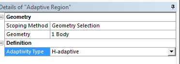
In metal forming and high-speed impact analyses, a body may experience very large amounts of plastic deformation. Single point integration explicit elements, which are usually robust for large deformations, may give inaccurate results in these situations due to inadequate element aspect ratios. To counteract this problem, LS-DYNA has the ability to automatically remesh a surface during an analysis to improve its integrity. This capability, known as adaptive meshing, is controlled with the adaptive region:
ℎ-adaptive for 3-D shells.
Passive ℎ-adaptive for 3-D shells. The elements in this part will not be split unless their neighboring elements in other parts need to be split more than one level.
Adaptive Solid to SPH creates SPH particles to either replace or supplement solid Lagrangian elements. Applications of this feature include adaptively transforming a Lagrangian solid part to SPH particles when the Lagrangian solid elements comprising those parts fail. One or more SPH particles (elements) will be generated for each failed element. The SPH particles replacing the failed solid Lagrangian elements inherit all the Lagrange nodal quantities (like displacement, velocity and acceleration) and all the Lagrange integration point quantities (like stress and strain) of these failed solid elements. Those properties are assigned to the newly activated SPH particles. The newly created SPH part can have different material properties using the Material Assignment field.
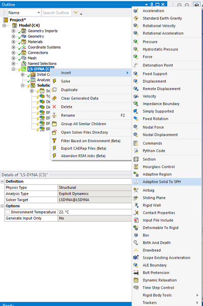
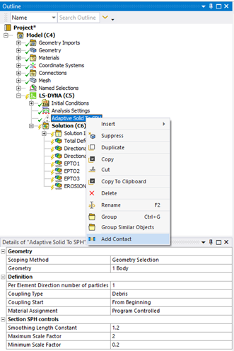
To insert an Adaptive Solid to SPH object, right-click LS-DYNA and select > as depicted in the following image.
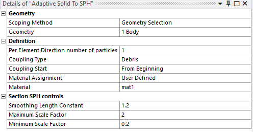
The input fields in the Details panel of Adaptive Solid to SPH are shown here.
You must scope this object to a solid part having a material compatible with SPH. Shell and beam elements are not allowed for this object. If you scope an object with an unsuitable material or geometry type, a warning message will be issued.
Adaptive Solid to SPH uses the keyword *DEFINE_ADAPTIVE_SOLID_TO_SPH.
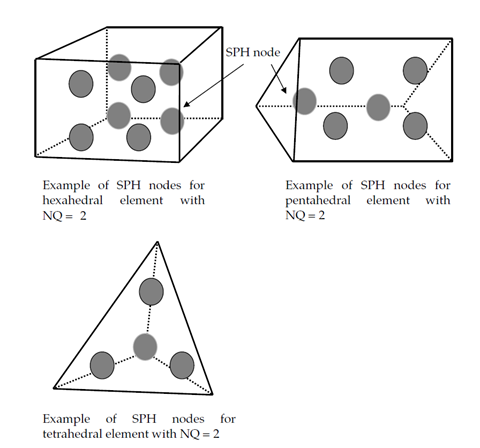
Per Element Direction number of particles is the number of SPH particles generated with respect to each direction of the solid element. This field sets the NQ parameter of the *DEFINE_ADAPTIVE_SOLID_TO_SPH keyword. For instance, when using hexahedral elements, the number of SPH particles generated inside a solid element for NQ=2 is 2*2*2=8 particles. For tetrahedral and pentahedral elements the number of particles is described in the following image.
Two options for the Coupling Type are available: Debris, and Coupled to Solid Element. This field is used for the ICPL parameter of the *DEFINE_ADAPTIVE_SOLID_TO_SPH keyword.
Two options for the Coupling Start are available: From Beginning, or When Solid Element Fails. This field is used for the IOPT parameter of the *DEFINE_ADAPTIVE_SOLID_TO_SPH keyword.
The newly created SPH part can have different material properties by setting Material Assignment in the Adaptive Solid to SPH object to User Defined, as shown in the previous Details panel image. All materials defined in Engineering Data are available in the Material field. When Material Assignment is set to Program Controlled, the SPH part will have the same material as the solid part.
For the SPH part created inside the solid part, the following Section fields are available and can be modified: Smoothing Length Constant, Maximum Scale Factor, and Minimum Scale Factor.
The SPH part is created inside the solver and is not visible in the Mechanical UI. Therefore, it can't be selected from the model tree if you want to scope the SPH part in a contact. To do this, add a new contact object under the Adaptive Solid to SPH object as shown in the following image. The contact object is inserted only when Material Assignment is set to User Defined.
This contact object allows you to define a contact between the SPH part created inside the solver (Contact Body) and Lagrangian parts (Target Bodies) that are visible in Mechanical as illustrated by the following figure.
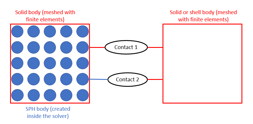
In the previous figure, Contact 1 is a surface-to-surface contact that can be defined with the manual contact region object. Contact 2 is a node-to-surface contact linking the inner solver SPH Part (Contact Body) to the segments of the Target Bodies (solid or shell).
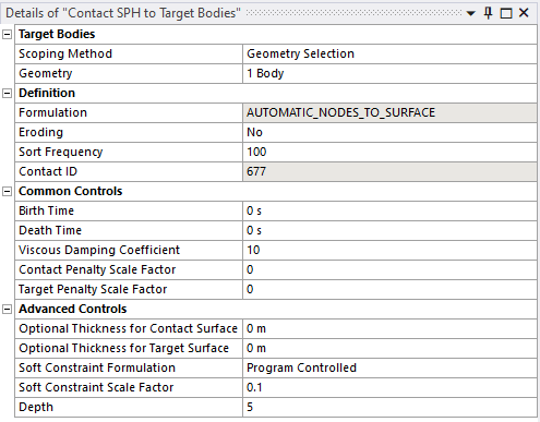
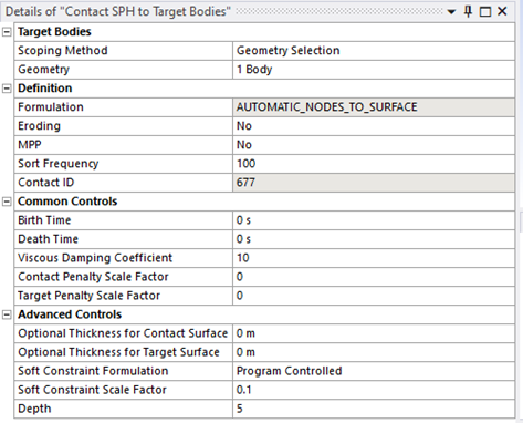
For the case of an SMP solution, the contact object properties would look as follows:
The following figure shows the contact properties when MPP is enabled for the analysis. You can choose not to use MPP for the contact calculation. Not using MPP for contact is sometimes more efficient.
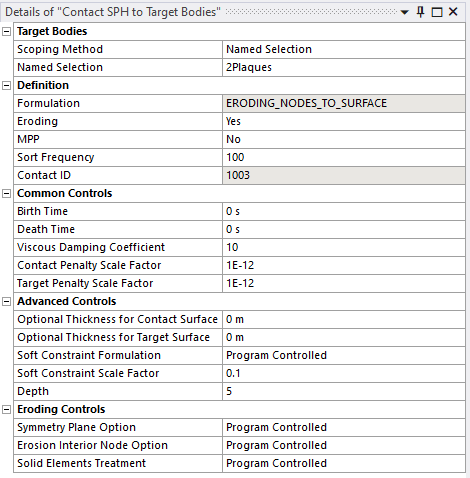
When Eroding is set to Yes, an additional block of input values appears as shown in the following figure:
You must define the target bodies for the contact. Two scoping methods are supported: Geometry Selection and Named Selection. Only solid and surface geometry selections are supported.
If you set Eroding to Yes, the card *CONTACT_ERODING_NODES_TO_SURFACE is written. When the property Eroding is set to No, the card *CONTACT_AUTOMATIC_NODES_TO_SURFACE is written.
The sort frequency corresponds to the parameter BSORT of Optional Card A in the case of SMP processing, and to the parameter BCKT of MPP Card 1 in the case of MPP processing.
Common Controls, Advanced Controls and Eroding Controls parameters are identical to the Contact Property object, and its definition can be found in Keywords Created from the Contact Properties Object.
This contact supports only Penalty and Soft Constraint formulations. The recommended formulation for an SPH simulation is the soft constraint (SOFT=1) and is used by default (Program Controlled).
When Material Assignment is set to Program Controlled and the scoped solid in the Adaptive Solid to SPH object is used in a manual contact region, a node-to-surface contact card is written between the SPH part (created inside the solver) and the target bodies. In other words, when Contact 1 (in the earlier figure) is defined, Contact 2 is written implicitly in the input file.
To view results on the created SPH particles, see Post-processing for Solver-Created SPH Elements.
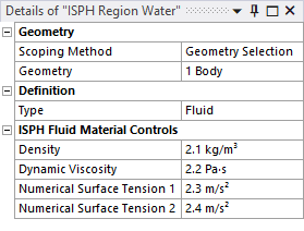
The Incompressible SPH (ISPH) solver allows you to solve FSI problems that involve Structural and Fluid bodies. This ISPH Region allows you to set the material properties for fluid and solid bodies. In addition, for solid bodies, the ISPH Region will mesh the interaction surface of the body with SPH particles and you can set the space between the SPH particles.
To set the material properties of the fluid part you must scope an ISPH Region object to the body, set the Type to fluid, and enter the material properties of the fluid.
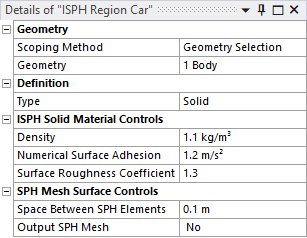
If a solid structural body is used in the model, you must extract its skin (using a modeling program like SpaceClaim) and define it as a new rigid shell body. The shell body should be meshed with triangles, then an ISPH Region should be scoped to the shell body. The interaction surface of the shell body is meshed with SPH particles using the ISPH Region. The ISPH Region will discretize the surface to SPH particles within the solver. Set the Type of the ISPH Region to Solid. You can then set the material properties for the solid, the space between the SPH elements, and whether you want to output the mesh to a file.
You can find information about Connections in Define Connections.
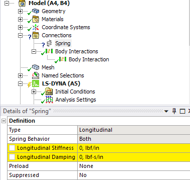
In LS-DYNA, Springs can be added in Connections. Both Longitudinal Stiffness and Damping are supported. For nonlinear springs, if you use Tabular Data to define the spring load curve, the force vs displacement curve must be defined with positive values for Spring Behavior set to Compression or to Tension. Negative values are valid only if the Spring Behavior is set to Both.
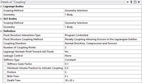
A Coupling object can be added under Connections to define the coupling mechanism used when modeling Fluid-Structure Interaction (FSI). The coupling object determines the interaction between the scoped Lagrange Bodies (those with Reference Frame set to Lagrange) and ALE bodies (those with Reference Frame set to S-ALE Domain or S-ALE Fill, or contained in a section definition with an ALE element formulation). The Coupling object creates an instance of either the *CONSTRAINED_LAGRANGE_IN_SOLID or the *ALE_STRUCTURED_FSI keyword in the solver input file. The field allows the keyword to be selected. The default Program Controlled option is *CONSTRAINED_LAGRANGE_IN_SOLID. The *ALE_STRUCTURED_FSI option is only applicable to S-ALE. Further information on the available options is given in the LS-DYNA Keyword User's Manual Volume I.
The Stiffness Type field allows you to define the stiffness as Constant (Stiffness Scale Factor) or Tabular (Penetration vs. Coupling Pressure).
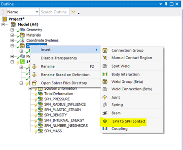
The SPH to SPH Contact object defines a penalty-based, node-to-node contact for particles of SPH parts. You can scope two SPH bodies that are interacting, and the solver will compute the interface stiffness value that guaranties stability (the interface stiffness is based on the nodal mass and the global time step size). This feature uses the keyword *DEFINE_SPH_TO_SPH_COUPLING and sets the parameter ISOFT to 1 (Soft constraint formulation).
To insert this object, right-click Connections and insert SPH to SPH Contact as shown here.
After the object is inserted, use the Details panel to scope a Contact body and a Target body.
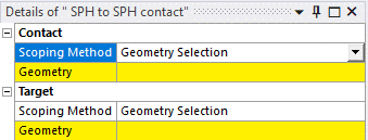
Scoping for this object is limited to SPH bodies and Adaptive Solid to SPH bodies. A warning message will be issued if incorrect scoping is attempted.
The ISPG to Surface Coupling object defines a tied coupling interface between fluid particles modeled with implicit smoothed particle Galerkin (ISPG) and a surface. The part selected must be ISPG or an error will occur. This feature writes the keyword *DEFINE_FP_TO_SURFACE_COUPLING.
To insert this object, right-click Connections and select > .
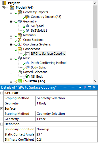
The Static Contact Angle is the angle between the surface and a tangent to the ISPG body passing through the contact point between the surface and ISPG body.
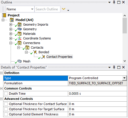
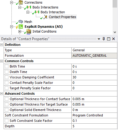
The Contact Properties object allows you to define LS-DYNA-specific contact options for a given Contact Region or a Body Interaction object. The object under analysis supersedes the object under Contact Region or Body Interaction if the two objects are scoped to the same contact.
Insert a Contact Properties object by right-clicking the contact you want to augment with LS-DYNA-specific properties, or by clicking the Contact Property icon on the LSDYNA Pre Tab.
 |
 |
You can also insert a Contact Properties object directly under an analysis environment. (You may want to do this in cases where you would like to have different properties for the same object in subsequent analyses). In this case, you can specify which contact you want the properties to apply to.
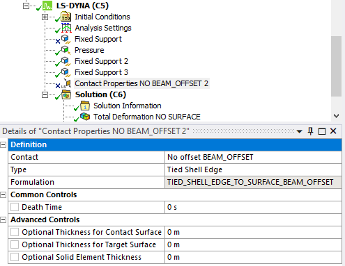
Note: You can right-click a Contact Properties object that is under an analysis environment and select Promote under Contact to move it to an existing contact or body interaction.
For more information on the options available through the Contact Properties object see Keywords Created from the Contact Properties Object.
You can find information about Mesh Settings in Apply Mesh Controls/Preview Mesh.
Dimensionally Reduced Rigid Body Behavior is not available for LS-DYNA.
The mesh for bodies with the Reference Frame S-ALE Domain is created within the solver. There are two methods that can be used to define the mesh parameters that are passed to the solver. The default method takes the number of mesh elements created by the Mechanical meshing process and calculates the number of divisions along each coordinate axis needed to obtain a uniform rectilinear mesh.

Where:
N = Number of elements in the Mechanical mesh
(dx , dy, dz) = Length of the bounding box of the body along each of the coordinate axes
(nx, ny, nz ) = The number of divisions along each of the co-ordinate axes
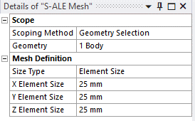
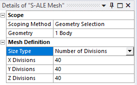
The second method is to insert an S-ALE Mesh object under the Model branch. This object can be scoped to the S-ALE Domain body, and either the element size or the number of divisions along each co-ordinate axis can be defined directly. The object also provides a visual representation of the mesh on the exterior surface of the body.
You can find information about creating a Named Selection in Named Selections in the Mechanical User's Guide.
The LS-DYNA Named Selection User ID field is only visible when a Named Selection object is created while performing an analysis using an LS-DYNA system in Workbench. This field allows you to define an id that will be used by the LS-DYNA solver for the named selection that you created. The value of the field can be:
0 - The id will be program controlled
Positive Integer - The number entered will be used by LS-DYNA as the id for the named selection
Note: If you read in an LS-DYNA input file that contains named selections, the LS-DYNA Named Selection User ID will not be set to the corresponding value for each Named Selection object created in the project. However, you can set the id of each named selection by hand if you change the Transfer PropertiesRead Only field in the Details panel of the Named Selection to No.
You can find information about Analysis Settings in Establish Analysis Settings.
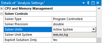
You can set Solver Precision to Single or Double under Solver Controls, or leave it as Program Controlled.
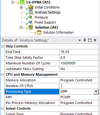
In LS-DYNA, the End Time is the only required input. SMP or MPP parallel processing can be activated by changing the Number of CPU's. Note that Ansys LS-DYNA HPC licenses are required for using more than 1 core.
The property Solver Units in the Solver Controls category has two options, Active System or Manual. If set to Active System the Solver Unit System property (which sets the solver unit system) will be read only and its value will determined by the GUI Unit System (set via the Units option in the Tools group of the Home tab on the ribbon). If set to Manual, the solver unit system can be set using the Unit System property and can be different from the GUI Unit System. This follows the standard Mechanical behavior described here.
SPH Controls
For the SPH solver, the following settings are available in the SPH Controls section of the Details panel in LS-DYNA. For more information, see *CONTROL_SPH.
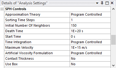
| Field | Description |
|---|---|
| Approximation Theory | Particle approximation method:
|
| Sorting Time Steps | Number of time steps between particle sorting |
| Initial Number of Neighbors | Initial number of neighbors per particle |
| Death Time | Death time for particle approximation |
| Start Time | Start time for particle approximation |
| Time Integration | Time integration type for the smoothing length:
|
| Maximum Velocity | Maximum velocity For SPH particles |
| Artificial Viscosity Formulation | Artificial viscosity formulation for SPH elements:
|
| Contact Thickness | If Yes, the solver will define a contact thickness in order to detect and avoid penetration between an SPH part and a Lagrangian part |
| Use Box | If Yes, exposes a Box Name field that lets you specify a standard boundary box to be used during the analysis |
ALE Controls
For the ALE solver, the following settings are available in the ALE Controls section of the Details panel in LS-DYNA. For more information, see *CONTROL_ALE.
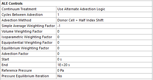
| Field | Description |
|---|---|
| Continuum Treatment | Flag to invoke alternate advection logic:
|
| Cycles Between Advection | Number of cycles between advections (almost always set to 1). |
| Advection Method | Advection methods:
|
| Simple Average Weighting Factor | ALE smoothing weight factor - Simple average |
| Volume Weighting Factor | ALE smoothing weight factor - Volume weighting |
| Isoparametric Weighting Factor | ALE smoothing weight factor - Isoparametric |
| Equipotential Weighting Factor | ALE smoothing weight factor - Equipotential |
| Equilibrium Weighting Factor | ALE smoothing weight factor - Equilibrium |
| Advection Factor | ALE advection factor (donor cell options, default = 1.0). This field is obsolete. |
| Start | Start time for ALE smoothing or start time for ALE advection if smoothing is not used. |
| End | End time for ALE smoothing or end time for ALE advection if smoothing is not used. |
| Reference Pressure | Applied to the free surfaces of the ALE domain. |
| Pressure Equilibrium Iteration | A flag to turn on or off the pressure equilibrium iteration option for multi-material elements. |