


To import loads for an analysis:
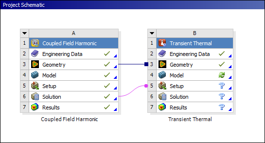
On the Workbench Project page, add the desired analysis that supports data transfer. Link the Solution cell of the upstream system to the Setup cell of the downstream system, as illustrated below. As required/desired, you can also link the Engineering Data and Geometry cells between the systems.
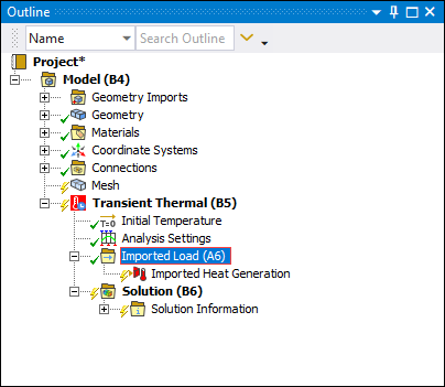
Double-click Setup cell of the downstream system to open the analysis in Mechanical. As illustrated in the following example, an Imported Load folder is automatically added under the environment folder. And, for this example, an Imported Heat Generation object was also automatically included in the folder.
To add an imported load, select the Imported Load folder and make a selection from the Environment Context tab. You can also right-click the folder, select , and add the desired load.
Note: Imported loads can be created using the option of the right-click context menu.
Based on the load definition, whether it has been mapped or if it is a newly inserted load, scope the loading condition to a geometric entity, mesh type, or to a geometry- or mesh-based Named Selection. Click when complete.
Note: Supported scoping options (geometric and/or mesh) vary based on the imported load type. For example, the following imported loads can be scoped to node-based Named Selections.
Imported Body Temperature (from External Data, for Submodeling [ not supported], or for Thermal-Stress)
Imported Displacement (from External Data or for Submodeling)
Imported Force (from External Data)
Imported Temperature (from External Data or for Submodeling)
Imported Velocity (from External Data)
Imported Initial Stress and Imported Initial Strain (from External Data), when the Apply To property is set to Corner Nodes
Set the appropriate options in the Details pane.
If you are transferring from Motion to a Harmonic Acoustics or Coupled Field Harmonic analysis, Fast Fourier Transform Controls properties will appear. These properties handle the parameters for the conversion of time-dependent source velocities to frequency-dependent velocities.
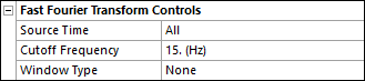
Source Time: Select the time domain from Motion to process. Options include or .
Cutoff Frequency: Select the highest frequency that can be obtained in the output of the conversion.
Note: Based on these two properties, the application will internally perform resampling on the time domain data to ensure evenly spaced data, optimize FFT performance and output frequency data up to the Cutoff frequency.
First, the minimum number of points is calculated using the maximum between (source_duration x cutoff_frequency x 2) and the initial number of points. The number of sampling points is then calculated by taking the next 2n value after the minimum number of points.
Window Type: Use this control to apply windowing to attenuate spectral leakage. Available options are as follows:
does not use a window for FFT.
uses windows of

uses windows of
 with
with 
uses windows of
 with
with 
uses windows of

uses windows of
 with
with 
uses windows of

uses windows of

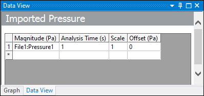
Use the Data View worksheet to control the load data that is imported. The imported values displayed in the worksheet, such as time, components, and magnitude, are based on the imported data type. The following example of Imported Pressure data displays Magnitude, Analysis Time, and options to specify Scale and Offset. The application displays similar worksheet data based on the imported load type.
Note:For Imported Temperature and Imported Body Temperature loads, the values used in the solution are calculated by first converting the imported load values into the solver unit system and then multiplying the scale value.
Specific transfer details can be found in the Special Analysis Topics section.
If you are using the Mechanical APDL solver, loads can be applied using tables or they can be applied at each analysis time/frequency specified in the imported load using the Tabular Loading property. When sending as tables, the loads can either be ramped or step changed (stepped) between the specified Analysis Times/Frequencies.
When ramped, the load value at step/sub-step is calculated using linear interpolation in the range where solve step/sub-step falls.
When stepped, the load value specified at t2 is applied in the range (t1, t2], where (t1, t2] is the range greater than t1 and less than or equal to t2.
Note:When program controlled, the loads are sent as tables when Analysis Time(s)/Frequency(ies) not matching any step end times/maximum frequency are present in the load definition. The loads are ramped for static/steady state and harmonic analyses and step applied for transient analyses.
Important: For an Imported Velocity object, when 1) the Tabular Loading property is set to , and 2) the Mapped Data property is set to , the application automatically applies the load as a ramped load for the harmonic analysis. See the Load Mapping Workflow Specification section for more information.
The loads are always sent as tables when Ramped or Stepped is chosen.
Important: Note that these options do not change the KBC command value (Key) which controls whether all of the loads within a load step are linearly interpolated or step changed. In addition, certain limitations apply to loads that do not support tabular loading, such as Imported Body Force Density. The limitations are described on the Help page for the respective loads.
Extrapolation is not performed when stepping/ramping the loads. If the solve time for a step/sub-step falls outside the specified Analysis Time/Frequency, then the load value at the nearest specified analysis time is used.
For temperature loads, the values are ramped from reference temperature for the first time step. For all other loads, the values are ramped from zero.
You can choose not to send the loads as tables using the Off option. The analysis times/frequencies specified in the load definition must match the step end times/maximum frequency in this case for the solution to succeed.
In a LS-DYNA analysis, the Off option is equivalent to the ramped option.
Import the load by right-clicking the Imported Load object and selecting Import Load.
When the load has been imported successfully, a contour or vector plot will be displayed in the Geometry window.
For vector loads types, contours plots of the magnitude (Total) or X/Y/Z component can be viewed by changing the Component property in the Details pane. Defaults to a vector plot (All).
For tensor loads types, contours plots of Equivalent (von-Mises) or XX/YY/ZZ/XY/YZ/ZX component can be viewed by changing the Component property in the Details pane. Defaults to a Vector Principal plot (All).
For Imported Convection loads, contours plots of film coefficient or ambient temperature can be viewed by changing the Component property in the Details pane.
For complex load types, such as pressure and velocity in Harmonic Response analyses, the real/imaginary component of the data can be viewed by changing the Complex Data Component option in the details pane.
The Legend controls options enable you to control the range of data displayed in the graphics window. By default, it is set to Program control, which allows for complete data to be displayed. If you are interested in a particular range of data, you can select the Manual option, and then set the minimum/maximum for the range.
Many imported loading conditions support Vector Display options.
Note:When you scope imported loading conditions to elements, you may see graphic artifacts on your model in the form of color "bleeding". Selecting the Wireframe option corrects the display.
The isoline option is drawn based on nodal values. When drawing isolines for imported loads that store element values (Imported Body Force Density, Imported Convection, Imported Heat Generation, Imported Heat Flux, Imported Pressure, Imported Surface Force Density, Imported Initial Stress and Imported Initial Strain), the program automatically calculates nodal values by averaging values of the elements to which a node is attached.
The minimum and maximum values of source data are also available in Legend Controls for External Data Import, Thermal-Stress, Submodeling, and Acoustic Coupling analyses.
To preview the imported load contour that applies to a given row in the Data View, use the Active Row option in the Details pane.
To activate or deactivate the load at a step, highlight the specific step in the Graph or Tabular Data window, and choose Activate/Deactivate at this step!. For additional rules when multiple load objects of the same type exist on common geometry selections, see Activation/Deactivation of Loads.
To export data, right-click the child load object and select > .