


This feature enables you to import fluid forces, pressures, temperatures, and convections from a steady-state or transient CFD analysis to a Mechanical application analysis.
This one-way transfer of face forces (tractions) or pressures at a fluid-structure interface enables you to investigate the effects of fluid flow in a static or transient structural analysis. Similarly, the one-way transfer of temperatures or convection information from a CFD analysis can be used in determining the temperature distribution on a structure in a steady-state or transient thermal analysis or to determine the induced stresses in a structural or LS-DYNA analysis.
To import loads from a CFD analysis:
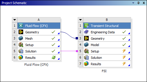
Complete your CFD analysis. From the Project Schematic, add an appropriate Mechanical analysis and create links between:
The Solution cell of your CFD analysis and the Setup cell of the newly added Mechanical or LS-DYNA analysis.
Your system should appear as illustrated here.
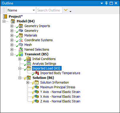
Double-click the Setup cell to open Mechanical. By default, an Imported Load folder is added under the Environment folder. Alternatively, select the Fluids Results File option of the Imported Loads drop-down menu on the Environment ribbon to manually insert an Imported Load (Fluids Results File) object to select an existing fluids results file from the disk.
Select the Imported Load (Group) object and:
Specify the Interpolation Type property as either: or (default).
Note: The option is not available for LS-DYNA analyses.
Right-click, select , and then select the desired load type you wish to add. Loads can also be added via the Environment Context Tab Imported Loads drop-down menu.
For your newly inserted load object, you can modify the following properties in the Definition category:
Tabular Loading: This property controls the creation and content of the Data View table. Data View values are applied at each load step. The options for this property include (default), , , .
Source Time: This property enables you to manage how the data from your source analysis is imported into the Data View table. The options for this property include (default), , and . Based on your selection, the time-based data contained in the Data View table displays accordingly.
Note:While defining source times and time step data, at any time you can right-click the imported load object and select the option . This option synchronizes the data of the Data View table with your Step Controls in the Analysis Settings object.
As needed, you can also change the values of the Source Time column entries in the Data View table. To do so, select a Source Time cell for the imported load in Data View table and specify a different value. Press Enter. The Source Time Step value changes based on the source time you select. If the selected source time corresponds to more than one source time step, you will also need to select the desired time step value. You can also change the Analysis Time and specify Scale and Offset values for the imported loads.
Source Time is not available for LS-DYNA analyses.
Limitation: For the setting, the Source Time field does not support non-zero values that are less than or equal to 1e-9s.
For your newly inserted load object, you can modify the following properties in the Transfer Definition category based on the setting of the Interpolation Type property. Note the following when making your specifications:
If you specify the Interpolation Type property as (default), refer to the Data Transfer Mesh Mapping section for detailed descriptions of the properties contained in the Settings, Graphics Controls, and Legend Controls categories.
Under the Transfer Definition category:
For surface transfer, open the drop-down menu for the CFD Surface property and select the corresponding CFD surface. If you have specified the Interpolation Type property as , you can use the Ctrl key to select multiple options from this menu.
For volumetric transfer, open the drop-down menu for the CFD Domain property and select the corresponding CFD Domain. If you have specified the Interpolation Type property as , you can use the Ctrl key to select multiple options from this menu.
For CFD Convection loads only: select the appropriate Ambient Temperature Type.
Note:
CFD Near-Wall Ambient (bulk) Temperature (default): This option uses the fluid temperature in the near-wall region as the ambient temperature for the film coefficient calculation. This value will vary along the face. When you specify as the Interpolation Type, Mechanical calculates the Wall Adjacent Heat Transfer Coefficient as the film coefficient. If you wish to use the Fluent derived heat transfer coefficients, export the solution data from Fluent and import it via External Data import.
Constant Ambient Temperature: This constant value applies to the entire scoped face(s). The film coefficient will be computed based on this constant ambient temperature value. Use of a constant ambient temperature value in rare cases may produce a negative film coefficient if the ambient temperature is less than the local face temperature. If this is the case, you can define a Supplemental Film Coefficient. This value will be used in place of the negative computed film coefficient and the ambient temperature adjusted to maintain the proper heat flow.
In a structural analysis, if the Imported Body Temperature load is scoped to one or more surface bodies, the Shell Face option in the details view enables you to apply the temperatures to Both faces, to the Top face(s) only, or to the Bottom face(s) only. See Imported Body Temperature for additional information.
In the Project Outline, right-click the imported load object and then select the Import Load option to import the load. When the load has been imported successfully, a contour plot will be displayed in the Geometry window.
Once the solution is complete for the Interpolation Type property set to , a CFD Load Transfer Summary is displayed as a Comment in the particular CFD load branch. The summary contains the following information:
For a CFD Pressure load: the net force, due to shear stress and normal pressure, on the face computed in CFD and the net force transferred to the Mechanical application faces. Note that Mechanical-Based Mapping only imports normal pressure.
For a CFD Temperature load: For surface transfers - the average computed temperature on the CFD boundary and the corresponding average mapped temperature on the Mechanical application faces.
For volumetric transfers – the average, maximum, and minimum temperature of the CFD domain and the corresponding Mechanical Application body selection(s).
For a CFD Convection load: the total heat flow across the face, and the average film coefficient and ambient temperature on the face.
The computed and mapped face data may be compared in order to get a qualitative assessment of the accuracy of the mapped data. Examples of the Imported Load Transfer Summary for the Interpolation Types are illustrated below.
| CFD Results Interpolator | Mechanical-Based Mapping |
|---|---|
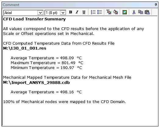 | 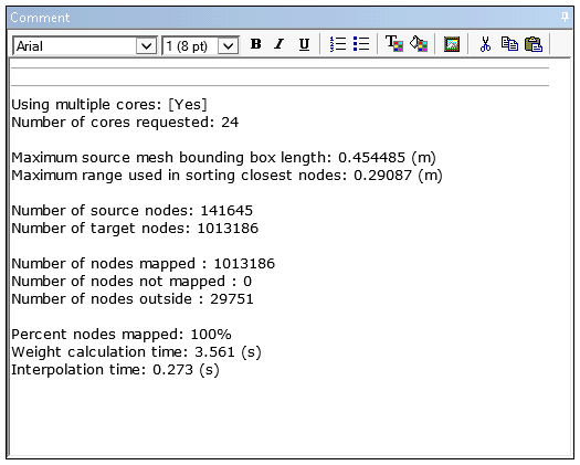 |
The following additional topics are covered in subsequent sections: