


You can find information about Results Processing in Review Results.
To collect Nodal Data, insert one or more Result Trackers under Solution prior to running the simulation. Result trackers must be scoped to a node.
Stress and Plastic Strain are written by default (can be suppressed) but Strain is not written by default and you must select it if desired.
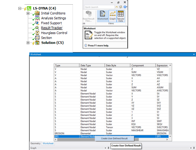
LS-DYNA keeps track of Total Strain and Plastic Strain. Elastic Strain will always show as 0. To plot elastic plastic strain or elastic strain, click Solution, then click Worksheet from the Home tab and select Available Solution Quantities within the Worksheet. Right-click the expression and select Create User Defined Result.
Time History Outputs (ASCII files) can be generated. All the files shown below can be created using the LS-DYNA system. Note however that some data in the ASCII files currently cannot be viewed.
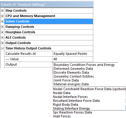
To view Time History Outputs select the ones desired from the ASCII drop-down menu.
Using LS-DYNA terminology, the following results can be viewed within LS-DYNA:
GLSTAT (Global Data : Kinetic Energy, Hourglass, ....).
BNDOUT (Boundary Conditions Data).
RCFORC (Contact Forces Data).
SPCFORC (Reaction Forces on Boundary Conditions) using *BOUNDARY_SPC (Fixed Support) to view Reaction Force.
MATSUM (Body Data).
NODOUT (Nodal Data) Trackers must be defined during pre-processing for the nodal data to be available during Results processing.
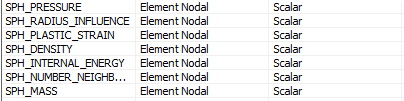
When an SPH body or an Adaptive Solid to SPH object is included in the model, several SPH-specific results are available as user defined variables. These results can be found in the worksheet as shown in the following images.
When using an Adaptive Solid to SPH object in the model, SPH particles are constructed inside the solver during the solution. To obtain results for these created SPH particles, do the following:
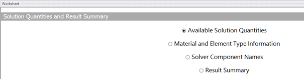
Access the worksheet, then select Material and Element Type Information as shown in the following figure:
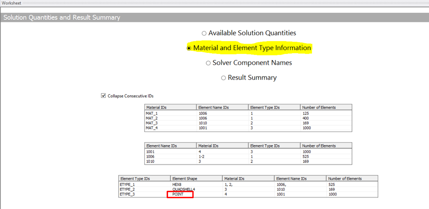
Locate the POINT element shape as depicted in the previous figure. By right-clicking the corresponding line, you can insert a total deformation result or any user-defined result. Remember that the available user-defined results can be viewed by selecting Available Solution Quantities on the worksheet.
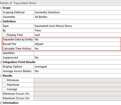
LS-DYNA allows you to store the results in a different file, which is separate from the main result file (d3plot). This file contains similar information, but is specifically for selected bodies or parts of the model. Since this file only contains results for a few bodies, the output frequency can be increased and more time steps can be stored in the result file.
Activate the output of the d3part file in Mechanical by setting Selective Output in Output Controls to Equally Spaced Points, or Time. If set to Equally Spaced Points, the Value field should be set to the number of time steps. If set to Time, the Value field should define a time interval between each output.
You must specify a named selection containing the bodies for inclusion in the d3part file using the Selective Output Scope field.

To display a particular result from the set of bodies selected for the d3part output, set Result File to d3part.
Explicit calculations often require thousands of calculation cycles. The result files typically contain a few dozens of these cycles.
Note: It is not possible to determine the maximum stress during the calculation. This could occur during unsaved cycles.
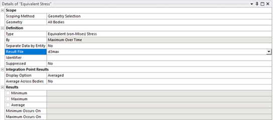
When you set Capture Maximum Stress Over Time in the Analysis Settings Output Controls category to Yes, LS-DYNA saves the maximum stress that occurred during the calculation. At each Capture Time, LS-DYNA compares the maximum stress to the previously saved value at each element of the mesh, and updates it if it increases.

The results are saved in the d3max file.
D3max results are only available for stress results. To display them, set By in the Definition category of the stress result to Maximum Over Time, and set Result File to d3max.
The Binout Result Tracker provides extensive access to the various results stored in the LS-DYNA result file binout.
To add a Binout Tracker, right-click the Solution Information object in the tree and select > .
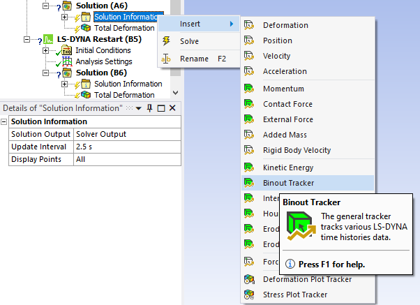
Binout is a binary file using the LSTC Data Archival Format or LSDA. This format mimics a Unix file system. Each result has the structure of a directory. It is called a Branch in the LSDA terminology. Each branch can have several subdirectories (sub-branches).
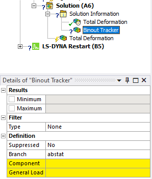
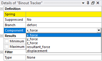
Each branch can have a number of components that allow you to access and plot the various results available for that branch.
The dbfsi data is available when ALE FSI Tracker Data is defined under Output Controls. FSI data is created for each Coupling object with the specified output frequency.

Mechanical supports the following Binout branches (Mechanical does not currently support all available components for each branch):
| abstat : Airbags results. |
| bndout: Boundary condition forces and energy results. |
| dbfsi: Fluid structure interaction data. |
| defgeo: Deformed geometry file results. |
| deforc: Discrete spring and discrete damper results. |
| elout: Elemental results. Mechanical defaults to and only supports elout beam or shell IP1 (Integration Point 1) results. |
| glstat: Global results. |
| jntforc: Joint results. |
| matsum: Part energies results. |
| nodout: Nodal translational motion results. |
| rbdout: Motion of rigid bodies in global and local coordinate systems. |
| rcforc: Resultant contact interface forces. |
| rwforc: Rigidwall forces. |
| secforc: Cross section forces. |
| sleout: Contact interface energies. |
| spcforc: Single point constraint reaction forces. |