


You can define the reference frame for bodies in an explicit dynamics analysis to be Lagrangian, Eulerian, or Particle. The following sections describe the reference frames and how their use affects the analysis.
By default, all bodies in an Explicit Dynamics analysis system are discretized and solved in a Lagrangian reference frame. The material associated with each body is discretized in the form of a body-fitted mesh. Each element of the mesh is used to represent a volume of material. The same amount of material mass remains associated with each element throughout the simulation. The mesh deforms with the material deformation. Solving using a Lagrangian reference frame is the most efficient and accurate method to use for the majority of structural models. However, in simulations where the material undergoes extreme deformations, such as in a fluid or gas flowing around an obstacle, the elements will become highly distorted as the deformation of the material increases. Eventually the elements may become so distorted that the elements become inverted (negative volumes) and the simulation cannot proceed without resorting to numerical erosion of highly distorted elements. The Explicit Dynamics solver offers two alternative solver formulations to overcome the problems of extreme deformations: the Eulerian and the Particle reference frames.
In an Eulerian reference frame, the grid remains stationary throughout the simulation. Material flows through the mesh. The mesh does not therefore suffer from distortion problems and large deformations of the material can be represented. If the material you are going to model is likely to experience very large deformations, using an Eulerian reference frame is therefore preferable.
Solving using an Eulerian reference frame is generally computationally more expensive than using a Lagrangian reference frame. The additional cost comes from the need to transport material from one cell to the next and also to track in which cells each material exists. Each cell in the grid can contain one or more materials (to a maximum of 5 in the Explicit Dynamics system). The location and interface of each material is tracked only approximately (to first order accuracy).
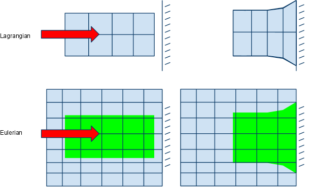
The representative example below shows a block of material impacting a rigid wall. First the block is represented in the Lagrangian reference frame. During the impact process the nodes of the mesh follow the deformation of the material. The same problem can be modelled in an Eulerian reference frame; here the nodes of the mesh are fixed in space, they do not move. Instead the material is tracked as it moves through the mesh.
Solid, Liquid and Gaseous materials can be used with an Eulerian (Virtual) reference frame in the Explicit Dynamics system. Because of the computational cost and approximate tracking of material interfaces, the Eulerian reference frame should be used only when very large deformation or flow of the material is expected.
The Particle reference frame uses a gridless technique for solving the computational continuum dynamics. In Explicit Dynamics, the gridless technique used is Smoothed Particle Hydrodynamics (SPH). SPH offers the following potential advantages over Lagrange and Euler processors:
SPH does not require a numerical grid
No grid tangling as in the Lagrange processor
No need for erosion
SPH is a Lagrangian technique
Allows efficient tracking of material deformation and history dependent behavior
Efficient compared with Eulerian techniques since only need to model regions where material exists, not where material will flow
Specific complex constitutive models can be included with relative ease compared with Eulerian techniques
Switching the reference frame of any solid body in a 3D Explicit Dynamics system, or a surface body in a 2D Explicit Dynamics system, from Lagrangian to Eulerian will result in the automatic creation of a virtual Multi-Material Eulerian domain. The domain will have properties such as dimensions and cell size determined by the Euler Domain Controls in the Analysis Settings. All solid bodies with the reference frame set to Eulerian will be mapped into the virtual Multi-Material Eulerian background grid at solve time and the material associated with these bodies will be solved for in the virtual Eulerian reference frame.
If one or more bodies have a reference frame set to Eulerian (Virtual), the following process is used on initialization to map the Euler bodies to a background Eulerian domain:
- Virtual Euler Domain
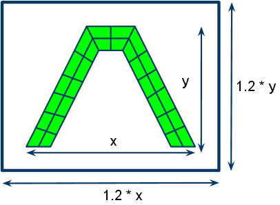
A background Eulerian (Virtual) domain is automatically generated to enclose all bodies in the model. By default, the domain size is set to 1.2 times the size of the bounding box of all bodies in the model. The domain is always aligned with the global Cartesian axes. Additional options to control the size of the domain are provided in the Analysis Settings.
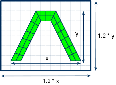
The background Euler domain is discretized with a mesh of uniform cell size. The cell size is defined to give approximately 500,000 cells in total. Additional options to control the cell size are provided in the Analysis Settings. The entire Euler domain is initialized as void; the cells contain no material.
- Mapping of Bodies with Euler Reference Frame to Virtual Euler Domain
The standard mesh generated on bodies marked with Eulerian (Virtual) reference frame is only used to represent the geometry of the body during initialization of the model for the solver. The material and initial conditions defined on bodies marked as Eulerian reference frame are mapped to the Euler domain. The mesh associated with the original body is then deleted, prior to the solve. A unique material is created for each body that is mapped into the Euler domain for the purposes of post processing.
If multiple bodies marked as Eulerian (Virtual) overlap, the body higher in the Outline view will take precedence. Therefore, the material assigned to the region of overlap will correspond to that assigned to the first Eulerian body.
The exterior faces of the Euler domain can each have one of three types of boundary condition applied. The type of boundary condition for each face is controlled in the Analysis Settings:
- Flow-out (Default)
This condition will allow any material reaching the boundary of the Euler domain to flow out of the domain at constant velocity.
- Rigid Wall
This condition makes the external boundaries of the domain act as a rigid wall.
- Impedance
This condition acts the same as a Flow-out condition and allows any material reaching the boundary of the Euler domain to flow out of the domain at constant velocity.
Key Concepts of Euler (Virtual) Solutions
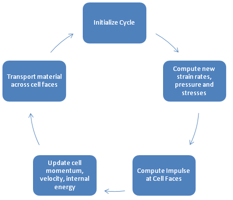
The conservation equations of mass, momentum and energy are solved on a block structured background mesh using a 2nd order accurate multi-material Godunov numerical scheme[17] with the second order upwind method by Van Leer [19, 20] for the 3D solver. The 2D Euler solver is first-order accurate. The computational cycle for bodies represented in an Eulerian reference frame is outlined below:
In comparison to a traditional Lagrangian numerical scheme, note the points in the following sections.
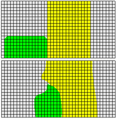
During the simulation, material can flow from one cell to another. At some stage in the computation a given cell is likely to contain more than one material. Note that void (free space) is also considered as a material in this sense; a cell containing one material and void is typical at any free surface of the material. In the example below we can see two solid materials (green and yellow) and free surfaces (white, void material) represented in an Eulerian reference frame.
A volume of fluid (VOF) method is used track the amount of material in each cell. Each material has a volume fraction and the sum of the volume fraction of each material, plus the volume fraction of void, will equate to unity.
 | (10–18) |
Nearly all isotropic material properties can be used in an Eulerian reference frame to represent solids, liquids or gases. Special treatment is required to allow calculation of the strain rates, pressure and stresses in each material in a cell, and also to calculate a resultant stress tensor which is then used to calculate cell face impulses, momentum and mass transport. Two algorithms are used for this purpose:
A cell containing two different gases; here we use an iterative procedure to establish an Equilibrium state (a density and energy of each gas which results in a uniform pressure across both gases).
A cell containing two or more non-gaseous materials; here we use a stiffness weighted averaging technique to distribute strain rates and establish the resultant pressure and deviatoric stress in each cell.
The choice of the above algorithms is automatic and local to each cell in the model.
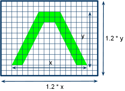
Important: At any point in time during the solution, only the volume fraction of each material in each cell is recorded and stored. The location of the material within the cell is not known. During post-processing of the model you will see an outline of the material displayed, this outline is an approximation derived from the volume fraction distribution in the cells. It is only accurate to within one cell dimension.
To move the solution through the mesh from one timestep to another, material must be transported across cell faces. If a cell contains only one material then we have a trivial solution and a volume fraction of that material will be transported across the face. If however we have multiple materials in a cell we need to employ an algorithm to decide which materials to transport and how much of each material to transport across each cell face. We are using the SLIC (Single Line Interface Construction) method [18] to calculate the order and quantity of material to transport across a cell face. This method takes information from both the upstream and downstream cells to make decisions on material transport.
A body with the reference frame set to Particle must be meshed with a Particle Method in Mechanical, which will generate a cloud of particles within the body. The continuum dynamics at those particles is solved for in Explicit Dynamics using the Smoothed Particle Hydrodynamics solver. The term Particle in Smoothed Particle Hydrodynamics is potentially misleading because the particles are really interpolation points. To demonstrate this point, consider a rod of steel that is represented by a series of SPH particles as illustrated in Figure 10.2: Particle Representation for Steel Bar.
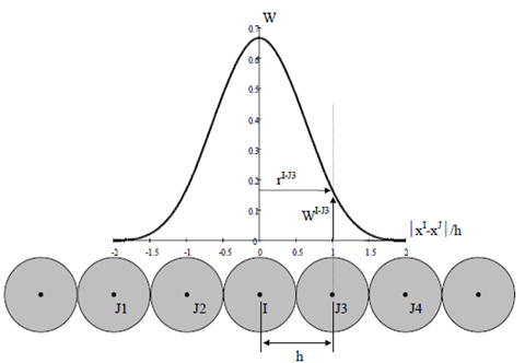
The density at particle I can be calculated using an expression such as
 | (10–19) |
Where mJ is the mass of particle J, WIJ is a weighting function, x is the position of the center of the particle, and h is the smoothing length (or particle diameter). In Explicit Dynamics, the default weighting function used is a Kernel B-spline. It is also possible to change the function to a quintic spline using a beta command snippet. To calculate the density of particle I, we sum the value of the density of all neighboring particles (interpolation points J1, J2, J3, J4, I) multiplied by the weighting function. A similar approach can also be taken to evaluate the value of other functions (for example strain rate) at particle I.
Hence, the SPH particles are not simply interacting mass points, but they are interpolation points from which values of functions and their derivatives can be estimated at discrete points in the continuum. In SPH, the discrete points at which all quantities are evaluated are placed at the center of the SPH particles. This is in contrast to the Lagrange processor where the interpolation points are defined at the corner nodes of each element, while the discrete points at which functions are evaluated are placed at the cell center (for density, strain rate, pressure, energy, stress) or the cell nodes (for displacement, velocity, force).
The computational cycle for SPH is similar to that for Lagrange except for some steps in which a Kernel approximation is used. This is shown in Figure 10.3: SPH Computational Cycle
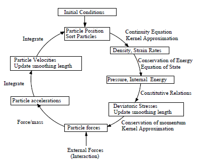
Kernel approximations are used to compute forces from spatial derivatives of stress and spatial derivatives of velocity are required to compute strain rates.