


The LS-DYNA and LS-DYNA Restart systems are available in the project Toolbox in Workbench. To run an LS-DYNA analysis, drag the system into a project and set up and run your model as usual. The LS-DYNA system will create an LS-DYNA keyword (.k) file that contains all the necessary information to carry out the analysis, and will run the LS-DYNA solver using that file.
For general information about setting up an Explicit Dynamics analysis, see Explicit Dynamics Workflow.
All the LS-DYNA keywords are implemented according to the LS-DYNA Keyword User's Manual Volumes I, II, III.
All the LS-DYNA keywords that are supported in Workbench are described in detail in Keywords used by LS-DYNA in Workbench. Any parameters that are not shown for a card are not used, and their default values will be assigned for them by the LS-DYNA solver.
When using Commands objects with LS-DYNA, be aware of the following:
Keyword cards read from Commands object content (renamed to Keyword Snippets for LS-DYNA) should not have any trailing empty lines if they are not intentional. This is because some keywords have more than one mandatory card that can be entered as blank lines, in which case the default values for the card will be used. Therefore, trailing blank lines should be used only if intended; otherwise they may cause solver execution errors.
The first entry in the Commands object content must be a command name which is preceded by the * symbol.
The most current released version of LS-DYNA is installed with your Ansys installation. You may install other versions of LS-DYNA and configure the software so that the other installed versions appear as options in the Analysis Settings (see Exposing Other Versions of LS-DYNA).
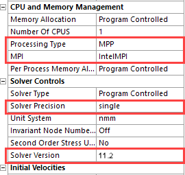
You can select the version of LS-DYNA that you want to run using the fields in the Analysis Settings. The following fields control the selection of the solver version:
- Processing Type
Choose whether to use the shared memory parallel processing (SMP), the massively parallel processing (MPP) capabilities of LS-DYNA, or choose Solve Process Settings.
With Solve Process Settings, the processing type is defined by the active setting in the Ribbon toolbar. If "Distributed" is checked, the solution will use MPP. If not, it will use SMP. For more information on Solve Process Settings, see the section Using Solve Process Settings in the Mechanical User's Guide.
If MPP is used, you must also choose the version of MPI that you want to use.
- Solver Precision
Choose whether to use Single or Double precision floating point representation.
- Solver Version
Choose the installed version of LS-DYNA that you want to use. See Exposing Other Versions of LS-DYNA for more information.
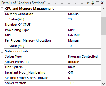
In addition to these settings, you can set up the memory allocation and parameters associated with LS-DYNA execution.
- Memory Allocation
Select Program Controlled for an automatic calculation of the required memory (MB) for the initialization of the analysis. The estimate is made from the number of nodes in the current model.
Select Manual to set your own memory size. Enter the size of the memory you want to use in the – Value[MB] field.
- Number of CPUs
Enter the number of CPUs that you want to use to run your job. For an SMP solution, if you enter the number of CPUs as a negative number, the job will run in a manner that will give you consistent results but will take longer.
To use the number of cores defined in the Ribbon toolbar as the Number of CPUs, choose Solve Process Settings for Processing Type and enter 0 for the Number of CPUs. For more information on Solve Process Settings, see the section Using Solve Process Settings in the Mechanical User's Guide.
- Per Process Memory Allocation
Select Program Controlled for an automatic calculation of the memory (MB) required for the analysis to run on each node. The same amount of memory will be allocated on each node.
Select Manual to set your own memory size. Enter the size of the memory you want to use in the – Value[MB] field.
If you have multiple versions of LS-DYNA installed on your system, you can choose to run any of them using the Solver Version field in the Analysis Settings. However, you must follow a procedure to allow Workbench to recognize that additional versions are installed.
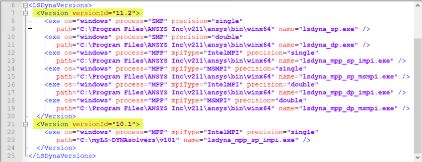
Each solver .exe file should be on your machine and the file lsdyna_solvers.xml must be properly defined. This file is created in the folder C:\Users\<CurrentUser>\AppData\Roaming\Ansys\242\ACTLSDYNA the first time that Ansys Mechanical is launched and recreated if it happens to be missing on subsequent launches. The content of the xml file before any modification, for a system running on Windows, should look as follows:
<?xml version="1.0" encoding="utf-8" standalone="yes"?>
<!--
File containing the default LSDyna solver files
Should contain at least one valid solver to prevent miscallaneous behavior
-->
<LSDynaVersions>
  <Version versionId="11.2">
    <exe os="windows" process="SMP" precision="single"
       path="C:\Program Files\ANSYS Inc\v242\ansys\bin\winx64" name="lsdyna_sp.exe" />
    <exe os="windows" process="SMP" precision="double"
       path="C:\Program Files\ANSYS Inc\v242\ansys\bin\winx64" name="lsdyna_dp.exe" />
    <exe os="windows" process="MPP" mpiType="IntelMPI" precision="single"
       path="C:\Program Files\ANSYS Inc\v242\ansys\bin\winx64" name="lsdyna_mpp_sp_impi.exe" />
    <exe os="windows" process="MPP" mpiType="MSMPI" precision="single"
       path="C:\Program Files\ANSYS Inc\v242\ansys\bin\winx64" name="lsdyna_mpp_sp_msmpi.exe" />
    <exe os="windows" process="MPP" mpiType="IntelMPI" precision="double"
       path="C:\Program Files\ANSYS Inc\v242\ansys\bin\winx64" name="lsdyna_mpp_dp_impi.exe" />
    <exe os="windows" process="MPP" mpiType="MSMPI" precision="double"
       path="C:\Program Files\ANSYS Inc\v242\ansys\bin\winx64" name="lsdyna_mpp_dp_msmpi.exe" />
  </Version>
</LSDynaVersions>
Note: The individual exe tags are shown on two lines so that they will be more readable. They will be one line in the file.
Every solver file must be uniquely defined by the following attributes:
- versionId
Solver version number, such as 11.2
- process
Process type, either SMP or MPP
- mpiType
The MPI type you want to use, such as IntelMPI (this field is only required when Process = MPP)
- precision
The solver precision you want to use, either single or double
These four attributes are used to create options that appear in the Analysis Settings fields of the LS-DYNA system in Workbench (see the following image).
Additional attributes of the exe tag complete the definition of
each solver option:
- os
Operating system of the machine on which LS-DYNA is running, either windows or linux
- path
Path (relative or absolute) of the folder containing the solver file
- name
Name of the solver file
If you want to solve with LS-DYNA versions that are not included in the
Ansys installation, you need to add a new Version tag in the xml
file, and one new exe tag per solver executable. The attributes
versionId, process (and mpiType if
the process is "MPP"), precision, os,
path and name are mandatory. In order for the
available options to appear in the UI drop-down menus and the solver files to
execute correctly, you must properly define these attributes.
The following example illustrates the necessary modifications to the xml file in order to include the single precision Intel MPI MPP solver from version 10.1.
After relaunching Mechanical, if you select the fields corresponding to the attributes of the newly defined solver entry, it will appear in the Solver Version menu, as in the following figure.
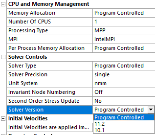
Note: Solver versions not included with the Ansys product distribution can be installed anywhere you like.
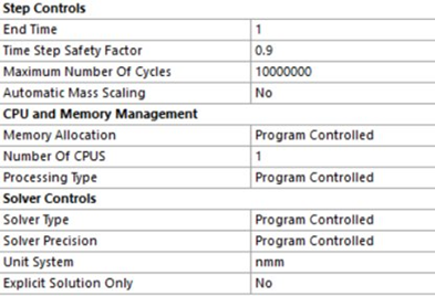
Use the Unit System field to set the units that the solver uses. All model inputs will be converted to this set of units during the solve. Results from the analysis will be converted back to the user's unit system in the GUI. For LS-DYNA systems, seven unit systems are available. These unit systems use the following base units:
- nmm
Metric (mm, tonne, N, s)
- μmks
Metric (µm, Kg, µN, s)
- Bft
US Customary (ft, lbm, lbf, s)
- Bin
US Customary (in, lbm, lbf, s)
- mks
Metric (m, Kg, N, s)
- cgs
Metric (cm, g, dyne, s)
- mm,ms,kg
Metric (mm, kg, kN, ms)
A sequential solution is an analysis technique that uses a combination of implicit (general Ansys or LS-DYNA) and explicit (LS-DYNA) solution methods. In problems that require a sequential solution, the results of an explicit analysis are imported into an implicit model (or vice-versa) for the purpose of obtaining a final solution.
Some of the reasons to perform a sequential solution include:
Some engineering processes are very complex and contain both dynamic and static phases (for example, initial hoop stress in a pressure vessel before a drop test or the linear elastic springback after sheet metal forming).
The explicit technique is geared towards solving nonlinear dynamic-impact problems and is not robust for solving static phases of physical phenomena.
The implicit method is best suited for solving static or quasi-static problems.
Combining implicit and explicit solvers is an extremely powerful tool for allowing simulations of otherwise intractable engineering problems.
The basic steps required to perform an explicit-to-implicit sequential solution include:
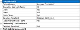
Solve the explicit portion of the analysis. Set the analysis option Stress File For Flexible Parts (saving the stresses on deformable parts) to Yes.
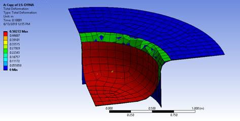
LS-DYNA will create a text file named dynain, which contains the deformed geometry along with the stresses on the deformable bodies. Displacements on rigid bodies are not saved in this file.
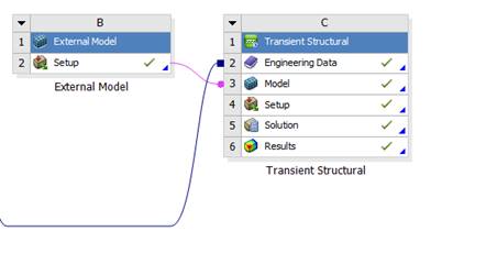
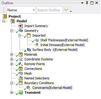
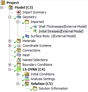
The dynain file is an LS-DYNA input file, which can be imported into a Mechanical system using the External Model component system. You must change the file's extension to .k before specifying the file in the External Model system. Link the External Model Setup cell to the Model cell of a Static Structural or Transient Structural system, or a LS-DYNA system if the deformed geometry and stresses are meant to be used in a subsequent LS-DYNA analysis.
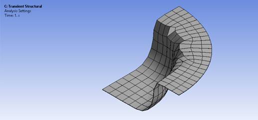
After you open the Mechanical Application you see that stresses, shell element thicknesses, and fixed displacement and fixed rotation constraints from the explicit analysis are imported into Mechanical.
Redefine the boundary conditions.
Solve the new analysis.
Additional Considerations for the LS-DYNA to Mechanical APDL Solver Workflow
If elasto-plastic materials are used in the explicit analysis, compatible elasto-plastic materials must be used in the subsequent Mechanical APDL analysis.
If the explicit analysis is using elasto-plastic materials, a minimum of five integration points should be used on shell elements if the subsequent analysis uses the Mechanical APDL solver. Additionally, an odd number of integration points for shell elements should be used in this workflow.
Limitations
The Mechanical APDL analysis relies on the initial state. Initial state does not support shear transfer on shell elements. If explicit stresses in the ZX and the YZ direction in the Mechanical APDL element coordinate system are significant, using this workflow is not recommended as Mechanical APDL will set the YZ and XZ shear to zero in all elements in their respective elemental coordinate system, regardless of the values imported from the .k file.
Mechanical APDL calculates the middle layer stresses using the top and bottom stresses by default. This can result in a difference in results. You can insert command snippets to import the value of the middle layer stresses from the external model file if necessary.
LS-DYNA Implicit features can also be used as an alternative to the Mechanical APDL solver, in the Implicit part of the workflow. The main benefit is that most of the LS-DYNA materials models are also available, and usable in the Implicit calculation.
To use LS-DYNA implicit features, set the option Explicit Solution Only to No.
Then set the following options:
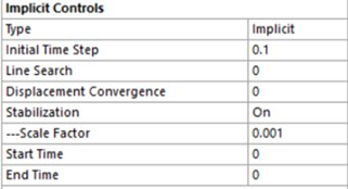
Initial Time Step: Initial time step size for implicit analysis
Line Search: Line search can be useful for enhancing convergence, but it can be expensive (especially with plasticity). You might consider setting Line Search on in the following cases:
When your structure is force-loaded (as opposed to displacement-controlled).
If you are analyzing a "flimsy" structure which exhibits increasing stiffness (such as a fishing pole).
If you notice (from the program output messages) oscillatory convergence patterns.
Displacement Convergence: Displacement convergence tolerance. This criteria controls the convergence on displacements. When the displacement norm ratio is below the displacement convergence, equilibrium is achieved. Small values will lead to a more accurate solution, at the expense of more iterations.
Stabilization: Convergence difficulty can happen when importing stresses from an explicit analysis into an implicit analysis. Nonlinear stabilization techniques can help achieve convergence. Nonlinear stabilization can be thought of as adding artificial dampers to all of the nodes in the system. Any degree of freedom that tends to be unstable has a large displacement causing a large damping/stabilization force. This force reduces displacements at the degree of freedom so that stabilization can be achieved.
There are two options for controlling stabilization:
Off (default): Deactivates stabilization.
On: Specifies stabilization should be used.
Scale Factor: Enter the scale factor value that the LS-DYNA solver uses to calculate stabilization forces.
Start Time: Enter the start time for the stabilization. Defaults to the beginning of the implicit calculation.
End Time: Enter the end time for the stabilization.