


*CONTROL_ACCURACY
Specifies control parameters that can improve the accuracy of the calculation.
Card
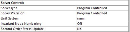
OSU is the global flag for objective stress updates. Required for parts that undergo large rotations. This value is set to 1 when the value of the Second Order Stress Update from the Solver Controls section of the Analysis Settings is set to On. Otherwise it is set to 0.
INN is the invariant node numbering for shell and solid elements. This value is set based on the Invariant Node Numbering from the Solver Controls section of the Analysis Settings .
= -4 if the Invariant Node Numbering is set to On for both shell and solid elements except triangular shells.
= -2 if the Invariant Node Numbering is set to On for shell elements except triangular shells.
= 1 if the Invariant Node Numbering is set to Off.
= 2 if the Invariant Node Numbering is set to On for shell and thick shell elements.
= 3 if the Invariant Node Numbering is set to On for solid elements.
= 4 if the Invariant Node Numbering is set to On for shell, thick shell, and solid elements.
*CONTROL_ALE
Inputs to this keyword are available in Analysis Settings object. Set global control parameters for the Arbitrary Lagrange-Eulerian (ALE) and Eulerian calculations.
Card 1
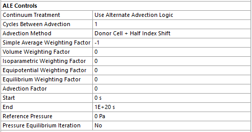
DCT = Flag to invoke alternate advection logic.
= -1 if the Continuum Treatment is set to Use Alternate Advection Logic (default).
<> -1 if the Continuum Treatment is set to Use Default Advection Logic.
NDV = Cycles Between Advection from the ALE Controls section of the Analysis Settings (Default to 1).
METH = Advection Method from the ALE Controls section of the Analysis Settings (Default to 1):
= 1 if the Advection Method is set to Donor cell + Half-Index-Shift.
= 2 if the Advection Method is set to Van Leer + Half-Index-Shift.
= -2 if the Advection Method is set to Van Leer (Relaxed Monotonicity).
= 3 if the Advection Method is set to Donor Cell (Total Energy Conservation).
= 6 if the Advection Method is set to Finite Volume With Flux Corrected Transport.
AFAC = Simple Average Weighting Factor from the ALE Controls section of the Analysis Settings. Smoothing weight factor - Simple average.
BFAC = Volume Weighting Factor from the ALE Controls section of the Analysis Settings. Smoothing weight factor - Volume Weighting
CFAC = Isoparametric Weighting Factor from the ALE Controls section of the Analysis Settings.
DFAC = Equipotential Weighting Factor from the ALE Controls section of the Analysis Settings.
EFAC = Equilibrium Weighting Factor from the ALE Controls section of the Analysis Settings.
Card 2
AAFAC = Advection Factor from the ALE Controls section of the Analysis Settings .
START = Start from the ALE Controls section of the Analysis Settings.
END = End from the ALE Controls section of the Analysis Settings.
PRIT = Pressure Equilibrium Iteration from the ALE Controls section of the Analysis Settings.
REF = Reference Pressure that is applied to the free surfaces of the ALE domain, from the ALE Controls section of the Analysis Settings.
*CONTROL_BULK_VISCOSITY
Sets the bulk viscosity coefficients globally.
Card
Q1 = 1.5. Quadratic Artificial Viscosity.
Q2 = 0.06. Linear Artificial Viscosity.
TYPE = -2. Internal energy dissipated by the viscosity in the shell elements is computed and included in the overall energy balance.
*CONTROL_CONTACT
Specifies the defaults for computations of contact surfaces.
Card 1
SLSFAC = 0 (uses the default = 0.1). Scale factor for sliding interface penalties.
RWPNAL = 0. Scale factor for rigid wall penalties. When equal to 0 the constrain method is used and nodal points which belong to rigid bodies are not considered.
ISLCHK = 1. Initial penetration check in contact surfaces. When set to 1 there is no checking.
SHLTHK = 1 (default). Shell thickness considered in surface to surface and node to surface contact types. When set to 1, thickness is considered but rigid bodies are excluded.
PENOPT = 1 (default). Penalty stiffness value option.
THKCHG = 0 (default).
ORIEN = 2. Automatic reorientation for contact segments during initialization. When set to 2 it is active for manual (segment) and automated (part) input.
ENMASS = 0. This parameter regulates the treatment of the mass for eroded nodes in contact. When set to 0 eroding nodes are removed from the calculation.
Card 2
USRSTR = 0. Storage per contact interface for user supplied interface control subroutine. When set to 0 no input data is read and no interface storage is permitted in the user subroutine.
Default values are used for all other parameters.
Card3
SFRIC = 0. Default static coefficient of friction.
Default values are used for all other parameters.
Card4
IGNORE = 2. Specifies whether to ignore initial penetrations in the *CONTACT_AUTOMATIC options. When set to 2 initial penetrations are allowed to exist by tracking them. Also, warning messages are printed with the original and the recommended coordinates of each contact node.
FRCENG = 1. Calculate frictional energy in contact. Convert mechanical frictional energy to heat when doing a coupled thermal-mechanical problem.
SKIPRWG = 0 (default).
OUTSEG = 1. Yes, output each beam spot weld contact node and its target segment for *CONTACT_SPOTWELD into D3HSP file.
SPOTSTP = 0 (default).
SPOTDEL = 1.Yes, delete the attached spot weld element if the nodes of a spot weld beam or solid element are attached to a shell element that fails and the nodes are deleted.
SPOTHIN = 0.5. This factor can be used to scale the thickness of parts within the vicinity of the spot weld. This factor helps avert premature weld failures due to contact of the welded parts with the weld itself. Should be greater than zero and less than one.
*CONTROL_ENERGY
Specifies the controls for energy dissipation options.
Card
HGEN = 2. Hourglass energy is computed and included in the energy balance. Results are reported in ASCII files GLSTAT and MATSUM.
RWEN = 2 (default).
SLNTEN = 2. Sliding interface energy dissipation is computed and included in the energy balance. Results are reported in ASCII files GLSTAT and SLEOUT.
RYLEN = 2. Rayleigh energy dissipation is computed and included in the energy balance. Results are reported in ASCII file GLSTAT.
*CONTROL_HOURGLASS
Defines the default values of the hourglass control type and coefficient. See *HOURGLASS for additional information.
Card
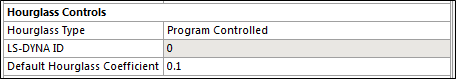
IHQ = Hourglass Type from the Hourglass Controls section of the Analysis Settings (Defaults to 1, Standard LS-DYNA Hourglass):
= 1 if the Hourglass Type is set to Standard LS-DYNA.
= 2 if the Hourglass Type is set to Flanagan-Belytschko Viscous Form.
= 3 if the Hourglass Type is set to Exact Volume Flanagan-Belytschko Viscous Form.
= 4 if the Hourglass Type is set to Flanagan-Belytschko Stiffness Form.
= 5 if the Hourglass Type is set to Exact Volume Flanagan-Belytschko Stiffness Form.
= 6 if the Hourglass Type is set to Belytschko-Bindeman.
= 7 if the Hourglass Type is set to Belytschko-Bindeman Linear Total Strain.
= 8 if the Hourglass Type is set to Full Projection Warping Stiffness.
QH = Default Hourglass Coefficient from the Hourglass Controls section of the Analysis Settings (Default to 0.1).
*CONTROL_IMPLICIT_SOLUTION
Controls the method used in implicit calculations.
ILIMIT is read from Iterations Per Reformation under the Implicit Controls section of the Analysis Settings.
= 0 (default) when Solution Method under the Implicit Controls section of the Analysis Settings is set to BFGS Slightly Nonlinear.
= 6 when Solution Method under the Implicit Controls section of the Analysis Settings is set to BFGS Moderately Nonlinear.
= 1 when Solution Method under the Implicit Controls section of the Analysis Settings is set to Full Newton.
Editable when Solution Method under the Implicit Controls section of the Analysis Settings is set to BFGS Custom.
MAXREF is read from Maximum Reformation under the Implicit Controls section of the Analysis Settings.
= 0 (default) when Solution Method under the Implicit Controls section of the Analysis Settings is set to BFGS Slightly Nonlinear
= 8 when Solution Method under the Implicit Controls section of the Analysis Settings is set to BFGS Moderately Nonlinear
= 30 when Solution Method under the Implicit Controls section of the Analysis Settings is set to Full Newton
< 0 (negative) when Force Convergence under the Implicit Controls section of the Analysis Settings is set to Yes
Editable when Solution Method under the Implicit Controls section of the Analysis Settings is set to Full Newton or BFGS Custom
RCTOL is read from Residual Relative under the Implicit Controls section of the Analysis Settings.
= 0 (default) & editable
ABSTOL is read from Absolute Tolerance under the Implicit Controls section of the Analysis Settings
= 0 (default) & editable
*CONTROL_IMPLICIT_SOLVER
Controls the linear equation solver.
LCPACK
= 0 (default) when Matrix assembly under the Implicit Controls section of the Analysis Settings is set to Symmetric Linear Solver
= 3 when Matrix assembly under the Implicit Controls section of the Analysis Settings is set to Nonsymmetric Linear Solver
*CONTROL_IMPLICIT_GENERAL
Activates implicit analysis and defines associated control parameters.
DT0 is read from Initial Time Step under the Implicit Controls section of the Analysis Settings.
= ENDTIM / 100 (default); ENDTIM is read from End Time in the Step Controls section of the Analysis Settings
*CONTROL_IMPLICIT_AUTO
Defines parameters for automatic time step control during implicit analysis.
DTMAX is read from Initial Time Step under the Implicit Controls section of the Analysis Settings.
= DT0 * 10 (default); ENDTIM is read from End Time in the Step Controls section of the Analysis Settings
*CONTROL_MPP_DECOMPOSITION_DISTRIBUTE_ALE_ELEMENTS
Ensures ALE elements are evenly distributed to all processors. The input card (with no parameters) is added by default, for MPP calculations. The input card will not be written if the property Distribute ALE Elements to All Processors is set to No in the ALE Controls section of the Analysis Settings object.
*CONTROL_MPP_IO_LSTC_REDUCE
Use LST's own reduce routine to consistently sum floating point data among processors. This keyword is written when all of the following conditions are met:
Processing Type under CPU and Memory Management is set to MPP
Explicit Solution Only under Solver Controls is set to No
Default Solver Controls Cards under Advanced is set to Keep
*CONTROL_MPP_IO_NOD3DUMP
Suppresses the output of the d3dump and runrsf files. This keyword is written when the following conditions are met:
Processing Type under CPU and Memory Management is set to MPP
Explicit Solution Only under Solver Controls is set to No
Default Solver Controls Cards under Advanced is set to Keep
Suppress Restart files for Distributed Calculations under Output Controls is set to Yes
*CONTROL_MPP_IO_NODUMP
Suppresses the output of all dump files and full deck restart files. This keyword is written when the following conditions are met:
Processing Type under CPU and Memory Management is set to MPP
Explicit Solution Only under Solver Controls is set to No
Default Solver Controls Cards under Advanced is set to Keep
Suppress Restart files for Distributed Calculations under Output Controls is set to Yes
*CONTROL_MPP_IO_NOFULL
Suppresses the output of the full deck restart files. This keyword is written when the following conditions are met:
Processing Type under CPU and Memory Management is set to MPP
Explicit Solution Only under Solver Controls is set to No
Default Solver Controls Cards under Advanced is set to Keep
Suppress Restart files for Distributed Calculations under Output Controls is set to Yes
*CONTROL_OUTPUT
This keyword controls the printing of various LS-DYNA output text files.
Card
NPOPT is the only parameter that is set. The value is set to 1. With that parameter set, nodal coordinates, element connectivities, rigid wall definitions, nodal SPCs, initial velocities, initial strains,adaptive constraints, and SPR2/SPR3 constraints are not printed.
*CONTROL_PARALLEL
Controls parallel processing usage for shared memory computers by defining the number of processors and invoking the optional consistency of the global vector assembly.
Card
CONST = 1. Consistency flag disabled for a faster solution
*CONTROL_SOLUTION
Specify the analysis solution procedure if thermal, coupled thermal analysis, or structural-only is performed.
Card
SOLN
= 0. Structural analysis only, if the Solver Type is set to Program Controlled or Structural Analysis Only.
= 2. Coupled structural thermal analysis, if the Solver Type is set to Coupled Structural Thermal Analysis.
*CONTROL_SHELL
Specifies global parameters for shell element types.
Card
WRPANG = 20 (default). Shell element warpage angle in degrees. If a warpage greater than this angle is found, a warning message is printed.
ESORT = 1, full automatic sorting of triangular shell elements to treat degenerate quadrilateral shell elements as C 0 triangular shells.
IRNXX = -1, shell normal update option. When set to -1, fiber directions are recomputed at each cycle.
ISTUPD = 4, shell thickness update option for deformable shells. Membrane strains cause changes in thickness in 3 and 4 node shell elements, however elastic strains are neglected. This option is very important in sheet metal forming or whenever membrane stretching is important. For crash analysis, setting 4 may improve energy conservation and stability.
THEORY = 2 (default). Belytschko-Tsay formulation.
BWC = 1. For this setting, Belytschko-Wong-Chiang warping stiffness is added.
MITER = 1 (default). Plane stress plasticity: iterative with 3 secant iterations.
PROJ = 1, the full projection method is used for the warping stiffness in the Belytschko-Tsay and Belytschko-Wong-Chiang shell elements. This option is required for explicit calculations.
NFAIL1 = 1. Flag to check for highly distorted under-integrated shell elements, print a message, and delete the element.
NFAIL4 = 1. Flag to check for highly distorted fully-integrated shell elements, print a message, and delete the element.
CNTO = 2. Flag to account for shell reference surface offsets in the contact treatment. Offsets are treated using the user defined contact thickness which may be different than the shell thickness used in the element.
*CONTROL_SOLID
Specifies global parameters for solid element types.
Card
ESORT = 1, full automatic sorting of tetrahedron and pentahedron elements to treat degeneracies. Degenerate tetrahedrons will be treated as ELFORM = 10 and pentahedron as ELFORM = 15 solids respectively (see *SECTION_SOLID).
*CONTROL_SPH
Provide controls relating to SPH solutions. Found in the Analysis Settings object Details panel.
Card
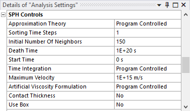
FORM = Approximation Theory value from the SPH Controls section of the Details panel as indicated below. The formulation stands for the method used to discretize the momentum equation.
=0: If set to Default Formulation or Program Controlled
=1: If set to Renormalization Approximation
=5: If set to Fluid Particle Approximation
=6: If set to Fluid Particle With Renormalization Approximation
=7: If set to Total Lagrangian Formulation
=8: If set to Total Lagrangian Formulation With Renormalization
=12: If set to Moving Least Squares
=13: if set to ISPH
=15: If set to Enhanced Fluid Formulation
=16: If set to Enhanced Fluid Formulation With Renormalization
Note: Moving Least Squares and ISPH are only available for an MPP simulation. You must set the processing type to MPP in the CPU and Memory Management section of the Details panel in order to use it.
NCBS = Sorting Time Steps from the SPH Controls section of the Details panel.
BOXID = ID of the box specified in Box Name in the SPH Controls section of the Details panel. Only Standard Box IDs are permitted in this field since SPH Boxes are selected automatically.
MEMORY = Initial Number of Neighbors value from the SPH Controls section of the Details panel. Defines the initial number of neighbors per particle. This parameter is used to determine the initial memory allocation for the SPH arrays.
DT = Death Time value from the SPH Controls section of the Details panel. Determines when the SPH calculations are stopped.
START = Start Time . Particle approximations will be computed when time of the analysis has reached the value defined in START.
DERIV = Time Integration value from the SPH Controls section of the Details panel. The smoothing length of each particle varies over time. Two types of equations can be used for the calculations.
=0: if set to Default or Program Controlled
=1: if set to Enhanced Energy Formulation
MAXV = Maximum Velocity value from the SPH Controls section of the Details panel. Particles with a velocity greater than MAXV are deactivated. A negative MAXV will turn off the velocity checking.
IAVIS = Artificial Viscosity Formulation value from the SPH Controls section of the Details panel. Defaults to 0.
=0: if set to Monaghan Formulation or Program Controlled
=1: Standard Formulation
*CONTROL_TERMINATION
Specifies the termination criteria for the solver.
Card
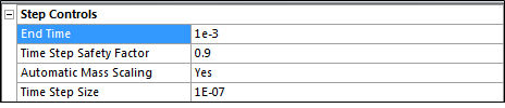
ENDTIM = End Time in the Step Controls section of the Analysis Settings .
ENDCYC = 10000000(constant) Maximum Time Steps .
DTMIN = 0.001 (constant).
ENDENG = 1000 (constant) Maximum Energy Error .
ENDMAS = 100000 (constant) Maximum Part Scaling .
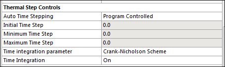
*CONTROL_THERMAL_TIMESTEP
This keyword is written if the simulation is determined to be a thermal one (for example, Coupled Structural Thermal Analysis). See Solver Type from the Solver Controls section of the Analysis Settings.
Card
TS = Auto Time Stepping from Thermal Step Controls (default to 1):
0 if Auto Time Stepping from Thermal Step Controls is set to No. The time step is fixed.
1 if Auto Time Stepping from Thermal Step Controls is set to Yes. The time step is variable (may increase or decrease).
TIP = Time integration parameter from Thermal Step Controls (default to Crank Nicholson Scheme TIP = 0):
0 if Time integration parameter from Thermal Step Controls is set to Crank-Nicholson scheme.
1 if Time integration parameter from Thermal Step Controls is set to Fully Implicit.
ITS = Initial Time Step from Thermal Step Controls.
TMIN = Minimum Time Step from Thermal Step Controls. If TMIN = 0.0, it is set to the structural explicit time step.
TMAX = Maximum Time Step from Thermal Step Controls. If TMAX = 0.0, it is set to 100 * the structural explicit time step.
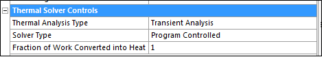
*CONTROL_THERMAL_SOLVER
This keyword is written if the simulation is determined to be a thermal one (for example, Coupled Structural Thermal Analysis). See Solver Type from the Solver Controls section of the Analysis Settings .
Card
ATYPE = Thermal Analysis Type from Thermal Solver Controls (default to 1)
0 if Thermal Analysis Type from Thermal Solver Controls is set to Steady State Analysis.
1 if Thermal Analysis Type from Thermal Solver Controls is set to Transient Analysis.
SOLVER = Solver Type from Thermal Solver Controls (defaults to 1):
1 if Solver Type is set to Symmetric Direct Solver.
2 if Solver Type is set to Nonsymmetric Direct Solver.
3 if Solver Type is set to Diagonal Scaled Conjugate Gradient Iterative.
4 if Solver Type is set to Incomplete Choleski Conjugate Gradient Iterative.
5 if Solver Type is set to Nonsymmetric Diagonal Scaled bi-Conjugate Gradient.
12 if Solver Type is set to Diagonal Scaling Conjugate Gradient Iterative.
13 if Solver Type is set to Symmetric Gauss-Siedel Conjugate Gradient Iterative.
14 if Solver Type is set to SSOR Conjugate Gradient Iterative.
15 if Solver Type is set to ILDLT0 Conjugate Gradient Iterative.
16 if Solver Type is set to Modified ILDLT0 Conjugate Gradient Iterative.
PTYPE = Thermal problem type from Thermal Nonlinear Controls.
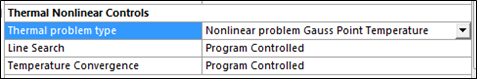
0 if Thermal problem type is set to Linear Problem.
1 if Thermal problem type is set to Nonlinear problem Gauss Point Temperature.
2 if Thermal problem type is set to Nonlinear problem Element Average Temperature.
FWORK = Fraction of Work Converted into Heat from Thermal Solver Controls (defaults to 1).
*CONTROL_THERMAL_NONLINEAR
This keyword is written if the simulation is determined to be a thermal one (for example, Coupled Structural Thermal Analysis). See Solver Type from the Solver Controls section of the Analysis Settings.
Card
THLSTL = Line Search from Thermal Nonlinear Controls (defaults to 0.0)
TOL = Temperature Convergence from Thermal Nonlinear Controls (defaults to 0.0).
*CONTROL_TIMESTEP
Specifies conditions for determining the computational time step.
Card
DTINIT = 0 Initial Time Step .
TSSFAC = Time Step Safety Factor from the Step Controls section of the Analysis Settings .
ISDO = 0 (default). Basis of time size calculation for 4-node shell elements.
TSLIMT = 0 Minimum Element Timestep ; the default value of 0.0 is used.
DT2MS = the negative value of Time Step Size specified in the Step Controls section of the Analysis Settings , if Automatic Mass Scaling is set to Yes . If Automatic Mass Scaling is set to No the default value of 0.0 is used.
LCTM = 0.
ERODE = 0 for an SPG analysis. An SPG analysis is recognized by having at least one Section object with Method set to SPG. If it is not an SPG analysis, then ERODE = 1 (constant). This field can't be changed from the user interface. It is set based on the analysis conditions.
MS1ST = 0 (default).
*DAMPING_GLOBAL
Specifies the mass weighted nodal damping applied globally to the nodes of deformable bodies and the center of mass of rigid bodies.
Card
LCID = 0, a constant damping factor will be used as specified in VALDMP.
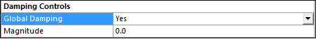
VALDMP = Magnitude from the Damping Controls section of the Analysis Settings (defaults to zero if Global Damping is set to No).
*CONTROL_IMPLICIT_GENERAL
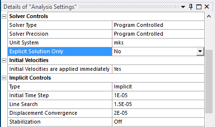
Setting Explicit Solution Only to No in the Solver Controls section of the Analysis Settings enables the use of the Implicit solver and displays the Implicit Controls section.
Card
DT0 is read from Initial Time Step under the Implicit Controls section of the Analysis Settings
IMFLAG = 1, to indicate an implicit analysis
*CONTROL_IMPLICIT_SOLUTION
Card
DCTOL is read from Displacement Convergence under the Implicit Controls section of the Analysis Settings
LSTOL is read from Line Search under the Implicit Controls section of the Analysis Settings
*CONTROL_IMPLICIT_SOLVER
Card
LPRINT = 1 (Linear solver print flag, controls screen and message file output)
*CONTROL_IMPLICIT_AUTO
Card
IAUTO = 1 (Automatic time step control flag)
*CONTROL_IMPLICIT_STABILIZATION
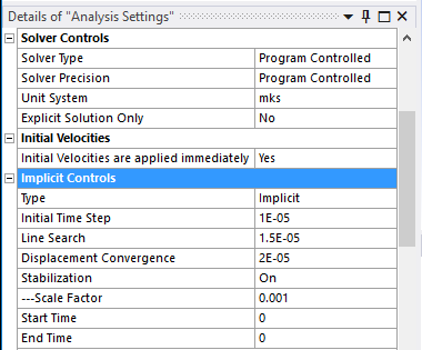
This keyword is written when Stabilization is set to On in the Implicit Controls section of the Analysis Settings
Card
IAS = 1 (to indicate the stabilization is active)
SCALE is read from –Scale Factor in the Implicit Controls section of the Analysis Settings
TSTART is read from Start Time in the Implicit Controls section of the Analysis Settings
TEND is read from End Time in the Implicit Controls section of the Analysis Settings