


Consider a coordinate system that is translating with a linear
velocity  and
rotating with angular velocity
and
rotating with angular velocity  relative to a stationary (inertial)
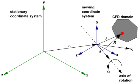
reference frame, as illustrated in Figure 2.3: Stationary and Moving Reference Frames. The origin of the moving
system is located by a position vector
relative to a stationary (inertial)
reference frame, as illustrated in Figure 2.3: Stationary and Moving Reference Frames. The origin of the moving
system is located by a position vector  .
.
The axis of rotation is defined by a unit direction vector  such that
 | (2–1) |
The computational domain for the CFD problem is defined with
respect to the moving frame such that an arbitrary point in the CFD
domain is located by a position vector  from the origin
of the moving frame.
from the origin
of the moving frame.
The fluid velocities can be transformed from the stationary frame to the moving frame using the following relation:
 | (2–2) |
where
 | (2–3) |
In the above equations,  is the relative velocity (the velocity viewed from
the moving frame),
is the relative velocity (the velocity viewed from
the moving frame),  is the absolute velocity (the velocity viewed from
the stationary frame),
is the absolute velocity (the velocity viewed from
the stationary frame),  is the velocity
of the moving frame relative to the inertial reference frame,
is the velocity
of the moving frame relative to the inertial reference frame,  is the translational frame
velocity, and
is the translational frame
velocity, and  is the angular velocity. It should
be noted that both
is the angular velocity. It should
be noted that both  and
and  can be functions of time.
When the equations of motion are solved in the moving reference frame, the acceleration of the fluid is augmented by additional terms that appear in the momentum equations [47]. Moreover, the equations can be formulated in two different ways:
Expressing the momentum equations using the relative velocities as dependent variables (known as the relative velocity formulation).
Expressing the momentum equations using the absolute velocities as dependent variables in the momentum equations (known as the absolute velocity formulation).
The governing equations for these two formulations will be provided in the sections below. It can be noted here that Ansys Fluent's pressure-based solvers provide the option to use either of these two formulations, whereas the density-based solvers always use the absolute velocity formulation. For more information about the advantages of each velocity formulation, see Choosing the Relative or Absolute Velocity Formulation in the User's Guide.
For the relative velocity formulation, the governing equations of fluid flow in a moving reference frame can be written as follows:
Conservation of mass:
 | (2–4) |
Conservation of momentum:
 | (2–5) |
where  and
and 
Conservation of energy:
 | (2–6) |
The momentum equation contains four additional acceleration
terms. The first two terms are the Coriolis acceleration ( ) and the centripetal acceleration
(
) and the centripetal acceleration
( ), respectively. These terms appear for both steadily
moving reference frames (that is, and are constant) and accelerating
reference frames (that is, and/or are functions of time). The third
and fourth terms are due to the unsteady change of the rotational
speed and linear velocity, respectively. These terms vanish for constant
translation and/or rotational speeds. In addition, the viscous stress
(
), respectively. These terms appear for both steadily
moving reference frames (that is, and are constant) and accelerating
reference frames (that is, and/or are functions of time). The third
and fourth terms are due to the unsteady change of the rotational
speed and linear velocity, respectively. These terms vanish for constant
translation and/or rotational speeds. In addition, the viscous stress
( ) is identical
to Equation 1–4 except that relative velocity
derivatives are used. The energy equation is written in terms of the
relative internal energy (
) is identical
to Equation 1–4 except that relative velocity
derivatives are used. The energy equation is written in terms of the
relative internal energy ( ) and the relative total enthalpy
(
) and the relative total enthalpy
( ), also known as the rothalpy.
These variables are defined as:
), also known as the rothalpy.
These variables are defined as:
 | (2–7) |
 | (2–8) |
For the absolute velocity formulation, the governing equations of fluid flow for a steadily moving frame can be written as follows:
Conservation of mass:
 | (2–9) |
Conservation of momentum:
 | (2–10) |
Conservation of energy:
 | (2–11) |
In this formulation, the Coriolis and centripetal accelerations
can be simplified into a single term ( ). Notice that the momentum equation
for the absolute velocity formulation contains no explicit terms involving
). Notice that the momentum equation
for the absolute velocity formulation contains no explicit terms involving  or
or  .
.
Ansys Fluent allows you to specify the frame of motion relative to an already moving (rotating and translating) reference frame. In this case, the resulting velocity vector is computed as
 | (2–12) |
where
 | (2–13) |
and
 | (2–14) |
Equation 2–13 is known as the Galilei transformation.
The rotation vectors are added together as in Equation 2–14, since the motion of the reference frame can be viewed as a solid body rotation, where the rotation rate is constant for every point on the body. In addition, it allows the formulation of the rotation to be an angular velocity axial (also known as pseudo) vector, describing infinitesimal instantaneous transformations. In this case, both rotation rates obey the commutative law. Note that such an approach is not sufficient when dealing with finite rotations. In this case, the formulation of rotation matrices based on Eulerian angles is necessary [544].
To learn how to specify a moving reference frame within another moving reference frame, refer to Setting Up Multiple Reference Frames in the User's Guide.