The DPM capabilities allow you to simulate moving particles as moving mass points, where abstractions are used for the shape and volume of the particles. Note that the details of the flow around the particles (for example, vortex shedding, flow separation, boundary layers) are neglected. Using Newton's second law, the ordinary differential equations that govern the particle motion are represented as follows:
 | (12–489) |
 | (12–490) |
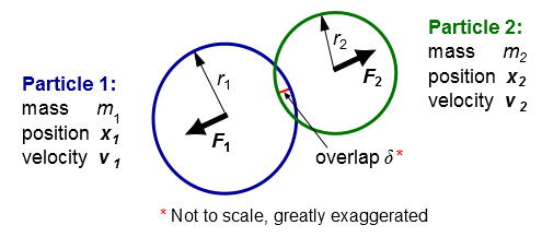
The DEM implementation is based on the work of Cundall and Strack [126], and accounts for the forces that result from
the collision of particles (the so-called "soft sphere"
approach). These forces then enter through the  term in Equation 12–489. The forces from the particle collisions are determined by the
deformation, which is measured as the overlap between pairs of spheres
(see Figure 12.27: Particles Represented by Spheres) or between a sphere and a boundary. Equation 12–489 is integrated over time to capture the
interaction of the particles, using a time scale for the integration
that is determined by the rigidity of the materials.
term in Equation 12–489. The forces from the particle collisions are determined by the
deformation, which is measured as the overlap between pairs of spheres
(see Figure 12.27: Particles Represented by Spheres) or between a sphere and a boundary. Equation 12–489 is integrated over time to capture the
interaction of the particles, using a time scale for the integration
that is determined by the rigidity of the materials.
The following collision force laws are available:
Spring
Spring-dashpot
Hertzian
Hertzian-dashpot
Friction
Rolling friction
The size of the spring constant of the normal contact force
for a given collision pair should at least satisfy the condition that
for the biggest parcels in that collision pair and the highest relative
velocity, the spring constant should be high enough to make two parcels
in a collision recoil with a maximum overlap that is not too large
compared to the parcel diameter. You can estimate the value of the
spring constant  using the following equation:
 | (12–491) |
where  is the parcel diameter,
  is the particle mass
density,
is the particle mass
density,  is the relative velocity between two colliding particles,
and
is the relative velocity between two colliding particles,
and  is the fraction of the diameter for allowable overlap. The collision
time scale is evaluated as
is the fraction of the diameter for allowable overlap. The collision
time scale is evaluated as  , where
  is the parcel mass (defined
by
is the parcel mass (defined
by  )
)
For the linear spring collision law, a unit vector ( ) is defined from particle 1
to particle 2:
) is defined from particle 1
to particle 2:
 | (12–492) |
where  and
and  represent the position of particle 1 and 2, respectively.
The overlap  (which is less than zero during contact) is defined
as follows:
(which is less than zero during contact) is defined
as follows:
 | (12–493) |
where  and
and  represent the radii of particle 1 and 2, respectively.
The force on particle 1 ( ) is then calculated using a spring constant
  that you define (and that
must be greater than zero):
that you define (and that
must be greater than zero):
 | (12–494) |
and then by Newton's third law, the force on particle 2 ( ) is:
) is:
 | (12–495) |
Note that  is directed away from particle 2, because
  is less than zero for
contact.
is less than zero for
contact.
The spring-dashpot collision law is a linear spring force law as described previously, augmented with a dashpot term described below.
For the spring-dashpot collision law, you define a spring constant  as in the spring collision
law, along with a coefficient of restitution for the dashpot term
(
as in the spring collision
law, along with a coefficient of restitution for the dashpot term
( ). Note that
  .
.
In preparation for the force calculations, the following expressions are evaluated:
 | (12–496) |
 | (12–497) |
 | (12–498) |
 | (12–499) |
 | (12–500) |
where  is a loss factor,
  and
and  are the masses of particle 1 and 2, respectively,
  is the so-called "reduced
mass",
is the so-called "reduced
mass",  is the collision time scale,
  and
and  are the velocities
of particle 1 and 2, respectively,
are the velocities
of particle 1 and 2, respectively,  is the relative
velocity, and
is the relative
velocity, and  is the damping coefficient. Note that
  , because
  .
.
With the previous expressions, the force on particle 1 can be calculated as:
 | (12–501) |
 is calculated using Equation 12–495.
The Hertzian collision law [240] is a nonlinear collision law. Using the same notations as in the section The Spring Collision Law, the force on particle 1 can be described as:
 | (12–502) |
Here, the constant  is calculated from the respective Young’s Moduli
  and
and  of the two colliding particles and their Poisson’s ratios
  and
and  :
:
 | (12–503) |
The Young’s Modulus has units of Pascals and is normally in the range of 1 GPa to a few 100 GPa. The Poisson ratio is a dimensionless constant in the range of -1 to 0.5.
 is calculated using Equation 12–495.
The Hertzian-dashpot collision law is a nonlinear collision force law as described in the section The Hertzian Collision Law augmented with the same dashpot term as in the linear spring-dashpot collision law (see The Spring-Dashpot Collision Law). That is, Equation 12–502 is modified as follows:
 | (12–504) |
 is calculated using Equation 12–495.
The friction collision law is based on the equation for Coulomb
friction ( ):
):
 | (12–505) |
where  is the friction coefficient and
  is the magnitude of the
normal to the surface force. The direction of the friction force is
opposite to the relative tangential motion, and may or may not inhibit
the relative tangential motion depending on the following:
is the magnitude of the
normal to the surface force. The direction of the friction force is
opposite to the relative tangential motion, and may or may not inhibit
the relative tangential motion depending on the following:
the size of the tangential momentum
the size of other tangential forces (for example, tangential components from gravity and drag)
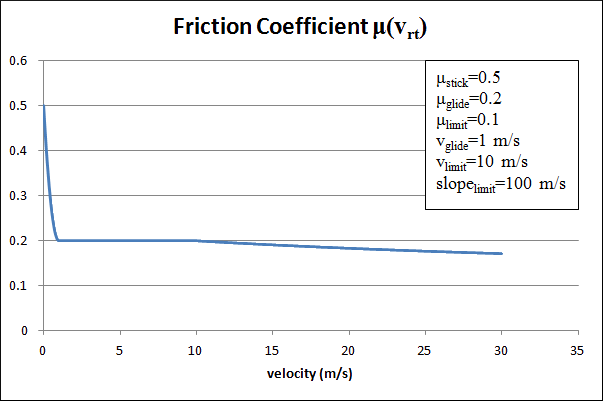
The friction coefficient is a function of the relative tangential
velocity magnitude ( ):
):
 :
:  :
:  :
:


|
where | |
|
| |
|
| |
|
| |
|
| |
|
| |
|
|


For an example of a plot of  , see Figure 12.28: An Example of a Friction Coefficient Plot.
The rolling friction collision law is an extension of the friction
collision law (The Friction Collision Law) based on
the equation for Coulomb friction ( ):
):
 | (12–506) |
where  is the rolling friction coefficient,
and
is the rolling friction coefficient,
and  is the magnitude of the force that is either normal
to the particle surface or pointing from one particle center to another.
The rolling friction force
is the magnitude of the force that is either normal
to the particle surface or pointing from one particle center to another.
The rolling friction force  acts only on the local torque at the particle-particle
or particle-wall contact point. This force may or may not inhibit
the relative angular velocity, depending on the size of the relative
torque.
acts only on the local torque at the particle-particle
or particle-wall contact point. This force may or may not inhibit
the relative angular velocity, depending on the size of the relative
torque.
For typical applications, the computational cost of tracking all of the particles individually is prohibitive. Instead, the approach for the discrete element method is similar to that of the DPM, in that like particles are divided into parcels, and then the position of each parcel is determined by tracking a single representative particle. The DEM approach differs from the DPM in the following ways:
The mass used in the DEM calculations of the collisions is that of the entire parcel, not just that of the single representative particle.
The radius of the DEM parcel is that of a sphere whose volume is the mass of the entire parcel divided by the particle density.
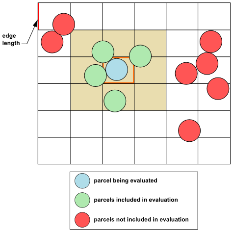
When evaluating the collisions between parcels, it is too costly
to conduct a direct force evaluation that involves all of the parcels.
Consider that for  parcels, the number of pairs that would need to
be inspected for every time step would be on the order of
parcels, the number of pairs that would need to
be inspected for every time step would be on the order of  . To address this issue, a geometric
approach is used: the domain is divided by a suitable Cartesian mesh
(where the edge length of the mesh cells is a multiple of the largest
parcel diameter), and then the force evaluation is only conducted
for parcels that are in neighboring mesh cells, because particles
in more remote cells of the collision mesh are a priori known to be out of reach. See Figure 12.29: Force Evaluation for Parcels for an illustration.
. To address this issue, a geometric
approach is used: the domain is divided by a suitable Cartesian mesh
(where the edge length of the mesh cells is a multiple of the largest
parcel diameter), and then the force evaluation is only conducted
for parcels that are in neighboring mesh cells, because particles
in more remote cells of the collision mesh are a priori known to be out of reach. See Figure 12.29: Force Evaluation for Parcels for an illustration.