


SHELL294
4-Node Thermal Shell
SHELL294 Element Description
SHELL294 is a 3D layered shell element having in-plane and through-thickness thermal conduction capabilities. The element has four nodes with no limitation on the number of interpolation layers (defined by through-thickness DOFs). It can also have several material layers per interpolation layer for a better balance between accuracy and computational load. The conducting shell element is applicable to a 3D, steady-state or transient thermal analysis. SHELL294 generates temperatures that can be passed to structural shell elements in order to model thermal bending. See SHELL294 in the Mechanical APDL Theory Reference for more details about this element. For verification examples, see VM97 and VM271 in the Ansys Mechanical APDL Verification Manual.
If the model containing the conducting shell element is to be analyzed structurally, use an equivalent structural shell element instead (SHELL181 or SHELL281).
Figure 294.1: SHELL294 Geometry
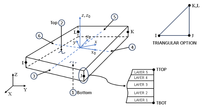
xo = element x-axis if ESYS is not supplied.
x = element x-axis if ESYS is supplied.
SHELL294 Input Data
The geometry, node locations, and coordinates systems for this element are shown in Figure 294.1: SHELL294 Geometry. The element is defined by four nodes, one thickness per layer, a material angle for each layer, and the material properties.
The cross-sectional properties are input using the SECTYPE,,SHELL and SECDATA commands. These properties are the thickness, material number, orientation of each layer, and number of integration points through the thickness of the layer. Real constants are not used for this element.
You can designate the number of integration points (1, 3, 5, 7, or 9) located through the thickness of each layer. Two points are located on the top and bottom surfaces respectively and the remaining points are distributed equal distance between the two points.
At each external node of the SHELL294 element, 3 DOFs are available including TEMP, TBOT, and TTOP when using D, DLIST, DDELE, IC, ICLIST, and ICDELE, and also when printing and plotting the nodal results using PRNSOL and PLNSOL. The other through-the-thickness DOFs are available to be printed and plotted by PRESOL, PLESOL, and *VGET.
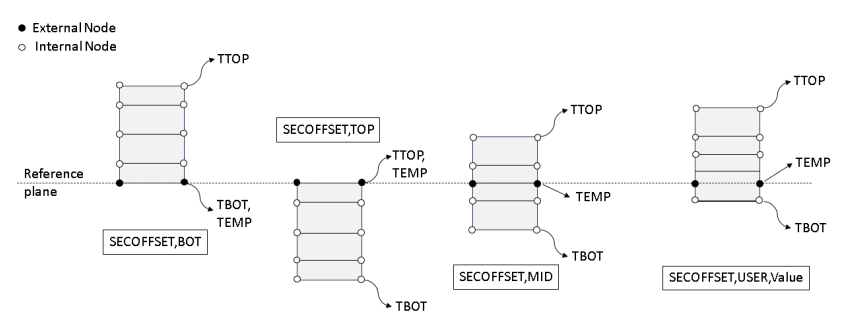
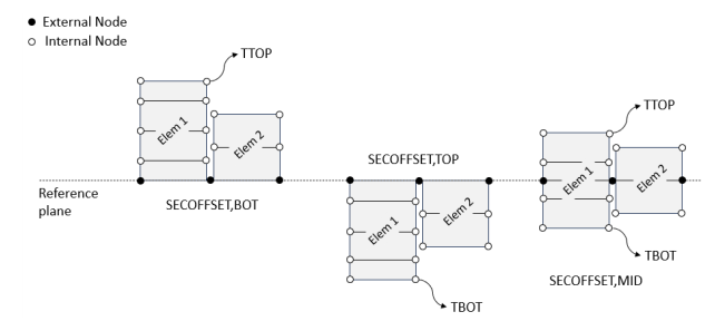
The TTOP and TBOT DOFs refer to temperatures at the top and bottom faces of SHELL294 respectively. The TEMP DOF refers to temperature at external node of SHELL294, which is located on the shell’s reference plane. The default location of the reference plane is at the middle, but it can be changed to the top, the bottom, or a user defined location defined by the SECOFFSET command. These cases are shown in the following figure. As can be seen, the TEMP DOF may have overlap with either TTOP or TBOT, depending on the section offset defined by SECOFFSET. For example, if the reference plane is on the bottom of the shell (SECOFFSET,BOT), then TBOT and TEMP are referring to the same DOF. In such cases of overlap between DOFs, the preference is generally given to TBOT/TTOP over TEMP. If, for example, both D,,TBOT and D,,TEMP are issued for a node of SHELL294 with SECOFFSET,BOT, then D,,TBOT takes priority over D,,TEMP.
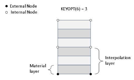
The material layers are defined via the SECDATA command. The number of material layers per interpolation layer is specified by KEYOPT(6). For example, by setting KEYOPT(6)=3, there will be 3 material layers per interpolation layer, and if there are 6 material layers in total, then there will be 2 interpolation layers in total, as shown in the following figure. The temperature varies linearly through the thickness within each interpolation layer. For the best accuracy, you can set KEYOP(6)=1, which means each material layer is modeled by an individual interpolation layer, but this can be computationally expensive, especially if the number of material layers is large. To lower the computational cost, you can set KEYOPT(6) to a number greater than 1 so that one interpolation layer encompasses several material layers, and the number of degrees of freedom is reduced.
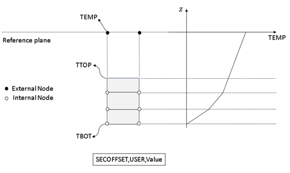
The reference plane can be located outside of the shell thickness when using SECOFFSET,USER,OFFSET, as shown in the following figure. In this situation, the temperatures at external nodes are calculated by extrapolating linearly from the interpolation layer on the top or bottom of the shell, depending on whether the reference plane is above or below it. As a result, if the reference plane is located outside the shell thickness, the temperature at external nodes may be noticeably different from the temperature variation through-the-thickness of the shell. The temperature at external nodes can be printed by PRNSOL,TEMP, and the temperature variation through-the-thickness of the shell can be printed by PRESOL,BFE,TEMP.
Other Input
The default orientation for this element has the S1 (shell surface coordinate) axis aligned with the element's first parametric direction at its center after being extruded in the thickness direction.
The default first surface direction S1 can be reoriented in the
element reference plane (as shown in Figure 294.1: SHELL294 Geometry) via the
ESYS command. You can further rotate S1 by angle
THETA (in degrees) for each layer via the SECDATA
command to create layer-wise coordinate systems. See Coordinate Systems for details.
Element loads are described in Element Loading. Convection or heat flux (but not both) and radiation (using the RDSF surface load label) may be input as surface loads at the element faces as shown by the circled numbers on Figure 294.1: SHELL294 Geometry. The surface loads are input on a per-unit-area basis at all 6 faces including shell edges. This is in contrast to SHELL131 where convection and flux loads on shell edges (faces 3 to 6) are input on a per-unit-length basis. Radiation is not available on the shell edges. You can also generate film coefficients and bulk temperatures using the surface effect element SURF152. SURF152 can also be used with FLUID116.
Heat generation rates may be input as element body loads on a per layer basis. One heat generation value is applied to the entire layer. If the first layer heat generation rate HG(1) is input, and all others are unspecified, they default to HG(1).
A summary of the element input is given in "SHELL294 Input Summary". A general description of element input is given in Element Input.
SHELL294 Input Summary
- Nodes
I, J, K, L
- Degrees of Freedom
TEMP - Material Properties
TB command: See Element Support for Material Models for this element. MP command: KXX, KYY, KZZ, DENS, C, ENTH - Surface Loads
- Convection or Heat Flux (but not both) --
Face 1 (I-J-K-L) (bottom, -z side) Face 2 (I-J-K-L) (top, +z side) Face 3 (J-I), Face 4 (K-J), Face 5 (L-K), Face 6 (I-L) - Radiation (using
Lab= RDSF) -- Face 1 (I-J-K-L) (bottom, -z side) Face 2 (I-J-K-L) (top, +z side) The surface loads can only be defined by the SFE command. If the reference plane is located on the bottom of the shell, then the surface loads on bottom can be defined by the SF command as well the SFE command. Similarly, if the reference plane is on top, then surface loads on top can be defined by the SF command as well as SFE command
- Body Loads
- Heat Generations --
HG(1), HG(2), HG(3), . . . ., HG(number of layers) Heat generation can be defined with the BFE command only.
- KEYOPT(2)
Evaluation of film coefficient:
- 0 --
Evaluate film coefficient (if any) at average film temperature, (TS+TB)/2
- 1 --
Evaluate at element surface temperature, TS
- 2 --
Evaluate at fluid bulk temperature, TB
- 3 --
Evaluate at differential temperature, |TS-TB|
- KEYOPT(6)
Number of material layers (>= 1) per interpolation layer:
- 1 --
Single material layer per interpolation layer (default)
- n --
n material layers per interpolation layer
- KEYOPT(8)
Material layer data storage:
- 0 --
Store data for bottom of bottom layer and top of top layer (default)
- 1 --
Store top and bottom data for all layers (the volume of data may be considerable).
- KEYOPT(10)
Through-the-thickness constraints:
- 0 --
Default value, user-defined temperature constraints, specified by the D command, can only be applied to top and bottom faces, but not on through-the-thickness DOFs.
- 1 --
If at any node, the temperature is specified by the D command on both the bottom and top faces, a linear variation through-the-thickness is enforced by the program on that node. This is done at the beginning of solve, at the first load step. Therefore, the temperature constraint on those nodes should not be altered between the load steps (for example, by the D or DDELE commands).
Note: If a node is shared between several SHELL294 elements and at least one of those elements has KEYOPT(10) = 1, then KEYOPT(10) = 1 applies to that node.
- KEYOPT(13)
Film coefficient matrix:
- 0 --
The program determines whether to use a diagonal or consistent film coefficient matrix (default).
- 1 --
Use a diagonal film coefficient matrix.
- 2 --
Use a consistent film coefficient matrix.
- KEYOPT(15)
Specific heat matrix:
- 0 --
The program determines whether to use a diagonal or consistent specific heat matrix (default).
- 1 --
Use a diagonal specific heat matrix.
- 2 --
Use a consistent specific heat matrix.
- KEYOPT(16)
This key option takes effect when adjacent elements have different layering. In that case, the DOFs from adjacent elements are constrained from bottom to top based on:
- 0 --
The geometry using hinge algorithm (the default behavior).
- 1 --
The DOF order (similar to SHELL131).
Note: If a node is shared between several SHELL294 elements and at least one of those elements has KEYOPT(16) = 1, then KEYOPT(16) = 1 applies to that node.
Different Layering in Adjacent Elements
When several SHELL294 elements with different layer configurations share a node, then the element with the largest thickness will represent TTOP and TBOT DOFs. Some examples with different values of section offsets are shown in the following figure.
All the options for section offset given by the SECOFFSET command are supported for SHELL294. The approximation space through the thickness is generally independent of the location of the reference plane. This means that in the absence of geometrical effects (for example, shell curvature), changing the section offset will not alter the solution. If the model is linear, the solution remains the same, and if there is nonlinearity, the converged solution should be the same by sufficiently tightening the convergence tolerance.
An exception to the above statement is when elements with different layering are adjacent to
each other, and the reference plane is located outside of at least one of those elements (via
SECOFFSET,USER,OFFSET). In that case, the results
can be different due to changes in approximation space, but this difference is expected to be
small in most cases, as described below.
The preceding discussion applies to the default value of KEYOPT(16) which is zero (hinge algorithm). If KEYOPT(16)=1, then SHELL294 behaves similar to SHELL131 in binding adjacent elements with different layering, and differences are expected to be seen for any change in section offset.
First, let’s consider the case of KEYOPT(16)=0 where the geometry is taken into account when binding adjacent elements with mismatched layers. In this case, if at a node, the reference plane passes through the element with smallest thickness (and therefore through all other elements sharing that node), then the approximation space will remain the same. This condition can be written as:

where  is the minimum thickness among all elements sharing a node, and
  is the user defined section offset by
SECOFFSET,USER,. If the reference plane is moved further up or down such that the above
condition is violated, then there is the possibility of having a different approximation space.
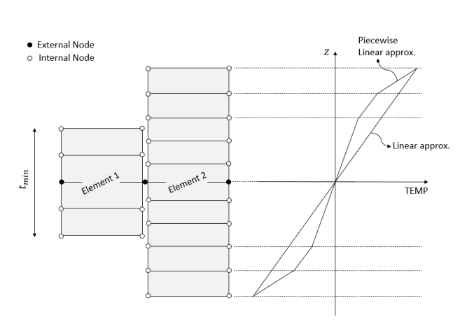
The amount of difference depends on the layer configuration of the elements. In general, the
largest difference that can happen is that the approximation space, which is originally piecewise
linear, is reduced to a single line from the bottom to the top of the shell, as depicted in the
following figure. In this figure, if
is the user defined section offset by
SECOFFSET,USER,. If the reference plane is moved further up or down such that the above
condition is violated, then there is the possibility of having a different approximation space.
The amount of difference depends on the layer configuration of the elements. In general, the
largest difference that can happen is that the approximation space, which is originally piecewise
linear, is reduced to a single line from the bottom to the top of the shell, as depicted in the
following figure. In this figure, if  , then the upper half will reduce to a single line, and if
  , then the lower half will reduce to a single line.
If the other option, KEYOPT(16)=1, is used, then SHELL294 behaves similar to SHELL131 in binding the adjacent elements with mismatched layers. In this case, the temperature at the bottom of adjacent elements are coupled together, and the same is done for the top of elements. Then all the DOFs in between are coupled based on their ordering when counted from the reference plane. In this case, for any change in the location of reference plane, there is a possibility of change in the approximation space. The option of KEYOPT(16)=1 is provided in consideration of the legacy behavior of SHELL131, and it is generally recommended that the new behavior of KEYOPT(16)=0 be used.
SHELL294 Output Data
The solution output associated with the element is in two forms:
Nodal temperatures included in the overall nodal solution (TEMP, TBOT, and TTOP)
Additional element output shown in Table 294.1: SHELL294 Element Output Definitions
Output temperatures may be read by structural shell elements SHELL181 and SHELL281 via the LDREAD,TEMP command.
Convection heat flux is positive out of the element; applied heat flux is positive into the element.
The element output directions are parallel to the layer coordinate system.
A general description of solution output is given in Solution Output. See the Basic Analysis Guide for ways to view results.
To see the temperature distribution through the thickness for this element, enter the POST1 postprocessor (/POST1), then issue /GRAPHICS,POWER and /ESHAPE,1 followed by PLESOL,BFE,TEMP.
The Element Output Definitions table uses the following notation:
A colon (:) in the Name column indicates that the item can be accessed by the Component Name method (ETABLE, ESOL). The O column indicates the availability of the items in the file jobname.out. The R column indicates the availability of the items in the results file.
In either the O or R columns, “Y” indicates that the item is always available, a letter or number refers to a table footnote that describes when the item is conditionally available, and “-” indicates that the item is not available.
Table 294.1: SHELL294 Element Output Definitions
| Name | Definition | O | R |
|---|---|---|---|
| EL | Element Number | Y | Y |
| NODES | Nodes - I, J, K, L | Y | Y |
| MAT | Material number | Y | Y |
| VOLU: | Volume | Y | Y |
| XC, YC, ZC | Location where results are reported | Y | 2 |
| HGEN | Heat generations HG(1), HG(2), HG(3),... | Y | - |
| TG:X, Y, Z | Thermal gradient components | Y | Y |
| TF:X, Y, Z | Thermal flux (heat flow rate/cross-sectional area) components | Y | Y |
| FACE | Face label | 1 | - |
| AREA | Face area | 1 | 1 |
| NODES | Face nodes | 1 | - |
| HFILM | Film coefficient at each node of face | 1 | - |
| TBULK | Bulk temperature at each node of face | 1 | - |
| TAVG | Average face temperature | 1 | 1 |
| HEAT RATE | Heat flow rate across face by convection | 1 | 1 |
| HEAT RATE/AREA | Heat flow rate per unit area across face by convection | 1 | - |
| HFAVG | Average film coefficient of the face | - | 1 |
| TBAVG | Average face bulk temperature | - | 1 |
| HFLXAVG | Heat flow rate per unit area across face caused by input heat flux | - | 1 |
| HFLUX | Heat flux at each node of face | 1 | - |
Available only at the centroid as a *GET item.
Table 294.1: SHELL294 Element Output Definitions lists output available through the ETABLE command using the Sequence Number method. See Element Table for Variables Identified By Sequence Number in the Basic Analysis Guide and The Item and Sequence Number Table in this reference for more information. The following notation is used in Table 294.2: SHELL294 Item and Sequence Numbers:
- Name
output quantity as defined in Table 294.1: SHELL294 Element Output Definitions
- Item
predetermined Item label for ETABLE command
- FCn
sequence number for solution items for element Face n
SHELL294 Assumptions and Restrictions
Zero area elements are not allowed. This occurs most frequently when the element is not numbered properly.
Zero thickness layers are not allowed.
A triangular element may be formed by defining duplicate K and L node numbers as described in Degenerated Shape Elements.
A free surface of the element (that is, not adjacent to another element and not subjected to a boundary constraint) is assumed to be adiabatic.
The full Newton-Raphson solution option (THOPT,FULL) must be used if thermal properties are defined via TB,THERM.
The Mass transport is not supported.
The tabular thickness specified by SECFUNCTION is not supported.
PRRFOR is not supported when adjacent elements have different layering. If the total force is requested (no FORCE command), then PRRSOL can be used instead.
With SECOFFSET,MID or USER, ramping forces from previous load step on deleted constraints (via DDELE,,,,,
RkeywithRkey= ON or FORCE) is not supported.General contact modeling technique is not supported for SHELL294. Only pair-based contact definition method is supported.
Among different contact elements, only CONTA174 and TARGE170 are currently supported. The KEYOPT(13) of CONTA174, intended for legacy SHELL131, is not applicable to SHELL294. The program identifies the shared DOF between contact/target and underlying SHELL294 automatically, based on face orientation. The
Tlaboption in ESURF,,Tlabcan be set to TOP or BOTTOM to generate contact and target elements with the intended orientation. Similarly, KEYOPT(11) of 3D thermal surface effect element, SURF152, intended for legacy SHELL131, does not apply to SHELL294. Again, ESURF,,TOP/BOTTOM can be used to generate SURF152 with the intended orientation, overlaid onto SHELL294.The through-the-thickness variation is always linear within an interpolation layer. The quadratic variation by adding midside nodes to the interpolation layers is not supported.
When applying a load on the edges of the shell (faces 3-6), the load is transferred to the top and bottom DOFs, TTOP/TBOT, as if there is only one interpolation layer and no through-the-thickness DOFs.
If an initial condition is supplied on both the bottom and top of the shell at any node, the program adds it to the through-the-thickness DOFs by assuming a linear variation from bottom to top.
The constrained node reaction solution, given by PRRFOR,HBOT/HTOP, refers to the heat at the bottom and top of the SHELL294 elements, produced only by this element type. In other words, if other element types (for example, SURF152) are attached to SHELL294, the heat from those element types are excluded from PRRFOR,HBOT/HTOP. In contrast, for PRRSOL,HBOT/HTOP, the heat from all element types are included in the HBOT/HTOP.
The constrained node reaction solution given by PRRFOR,HBOT/HTOP, and the element data stored by ESOL,,,HBOT/HTOP, refer to the heat at the bottom and top of the shell. If heat is nonzero at some middle nodes, between the bottom and top, then the program sums the heat at those middle nodes, and adds half of the sum to the bottom, HBOT, and the other half to the top, HTOP. Therefore, the summation of HBOT and HTOP gives the total heat through-the-thickness of the shell from bottom to top.
The constrained node reaction solution, given by PRRSOL,HBOT/HTOP, refers to the heat at the bottom and top of the shell. If the reference plane is located at either of those two locations, then the corresponding HBOT/HTOP refers to the heat at the external node of the shell located on the reference plane.
PRRSOL,HBOT and RFORCE,,,HBOT are not available if the reference plane is located inside the bottom layer, or below the bottom of the shell. Similarly, PRRSOL,HTOP and RFORCE,,,HTOP are not available if the reference plane is located inside the top layer, or above the top of the shell. If the reference plane is located inside any other layer, or exactly at the bottom or top or the interface between two adjacent layers, then all those data are available. If PRRSOL is not available, you can use PRRFOR instead.
Defining constraint equations by CE and coupled sets by CP are not supported for TBOT and TTOP of SHELL294 elements.
Nonlinear material properties are evaluated at each integration point.