


The following additional POST1 postprocessing techniques are covered in this section:
- 7.3.1. Rotating Results to a Different Coordinate System
- 7.3.2. Performing Arithmetic Operations Among Results Data
- 7.3.3. Creating and Combining Load Cases
- 7.3.4. Mapping Results onto a Different Mesh or to a Cut Boundary
- 7.3.5. Creating or Modifying Results Data in the Database
- 7.3.6. Splitting Large Results Files
- 7.3.7. Magnetics Command Macros
- 7.3.8. Comparing Nodal Solutions From Two Models or From One Model and Experimental Data (RSTMAC)
Results data, calculated during solution, consist of displacements (UX, UY, ROTX, etc.), gradients (TGX, TGY, etc.), stresses (SX, SY, SZ, etc.), strains (EPPLX, EPPLXY, etc.), etc. These data are stored in the database and on the results file in either the nodal coordinate system (for the primary, or nodal data) or the element coordinate system (for the derived, or element data). However, results data are generally rotated into the active results coordinate system (which is by default the global Cartesian system) for displays, listings, and element table data storage.
Using the RSYS command, you can change the active results
coordinate system to global cylindrical (RSYS,1), global
spherical (RSYS,2), any existing local coordinate system
(RSYS,N, where
N is the local coordinate system number),
or the nodal and element coordinate systems used during solution
(RSYS,SOLU). If you then list, display, or operate on the
results data, they are rotated to this results coordinate system first. You may also
set the results system back to global Cartesian (RSYS,0).
The default coordinate system for certain elements, notably shells, is not global Cartesian and is frequently not aligned at adjacent elements.
The use of RSYS,SOLU with these elements can make nodal averaging of component element results, such as SX, SY, SZ, SXY, SYZ, and SXZ, invalid and is not recommended.
The following figure illustrates how displacements are reported for several different RSYS settings:

The displacements are in terms of the nodal coordinate systems (which are always Cartesian systems), but issuing the RSYS command causes those nodal systems to be rotated into the specified system. For example, RSYS,1 causes the results to be rotated parallel to the global cylindrical system such that UX represents a radial displacement and UY represents a tangential displacement. (Similarly, VX and VY in a fluid analysis are reported as radial and tangential values for RSYS,1.)
Caution: Certain element results data are always output in the element coordinate system regardless of the active results coordinate system. These are miscellaneous result items that you would normally expect to be interpreted only in the element coordinate system. They include forces, moments, stresses, and strains for beam, pipe, and spar elements, and member forces and moments for some shell elements.
In most circumstances, such as when working with a single load case or during linear combinations of multiple load cases, rotating results data into the results coordinate system does not affect the final result values. However, most modal combination techniques (PSD, CQC, SRSS, etc.) are performed in the solution coordinate system and involve squaring operations. Since the squaring operation removes the sign associated with the data, some combined results may not appear as expected after being rotated into the results coordinate system. In these cases, RSYS,SOLU is on by default in order to keep the results data in the solution coordinate systems. No other coordinate system may be used.
As an example of when you would need to change the results coordinate system, consider the case of a cylindrical shell model, in which you may be interested in the tangential stress results. The SY stress contours before and after results coordinate system transformation are shown below for such a case.
PLNSOL,S,Y           ! Display a: SY is in global Cartesian system (default)
RSYS,1
PLNSOL,S,Y           ! Display b: SY is in global cylindrical system
See the RSYS and PLNSOL command descriptions for further information.
Figure 7.19: SY in Global Cartesian and Cylindrical Systems
Plot 1 (top) illustrates SY in global Cartesian system. Plot 2 (bottom) illustrates SY in global cylindrical system (note that nodes and elements are still in global Cartesian system).
In a large-deformation analysis (NLGEOM,ON), the element coordinate system is first rotated by the amount of rigid body rotation of the element. Therefore, the component stresses and strains and other derived element data include the effect of the rigid body rotation. The coordinate system used to display these results is the specified results coordinate system rotated by the amount of rigid body rotation.
The exceptions to this are continuum elements such as PLANE182, PLANE183, SOLID185, SOLID186, SOLID187, SOLID272, SOLID273, and SOLID285. For these elements, the output of the element component results is by default in the initial global coordinate system, and all component result transformations to other coordinate systems will be relative to the initial global coordinate system.
The primary data (for example, displacements) in a large-deformation analysis do not include the rigid body rotation effect, because the nodal coordinate systems are not rotated by the amount of rigid body rotation.
The earlier discussion of operations among path items was limited to items mapped on to a path. Using commands from the POST1 CALC module, you can perform operations among any results data in the database. The only requirement is that you must use the element table. The element table serves as a "worksheet" that allows arithmetic operations among its columns.
The procedure to do calculations among results data requires three simple steps:
The ETABLE command moves specified results data for all selected elements into the element table. One value is stored per element. For example, if you select 10 elements and issue the command shown below, an average UX value is calculated for each element from the nodal displacements and stored in the element table under the "ABC" column.
ETABLE,ABC,U,X
The element table will be ten rows long (because only ten elements were selected). If you now want to double these displacements, the command (SMULT) to do so is:
SMULT,ABC2,ABC,,2
The element table now has a second column, labeled ABC2, containing twice the values in column ABC. To list the element table, simply choose PRETAB.
Example 7.13: PRETAB Output
PRINT ELEMENT TABLE ITEMS PER ELEMENT
***** POST1 ELEMENT TABLE LISTING *****

   STAT    CURRENT     CURRENT
   ELEM    ABC         ABC2
      1   .21676      .43351
     11   .27032      .54064
     21   .23686      .47372
     31   .47783      .95565
     41   .36171      .72341
     51   .36693      .73387
     61   .13081      .26162
     71   .50835      1.0167
     81   .35024      .70049
     91   .25630      .51260
MINIMUM VALUES ELEM 61 61 VALUE .13081 .26162
 MAXIMUM VALUES
 ELEM        71          71
 VALUE    .50835      1.0167
Another example of arithmetic operations is to calculate the total volume of selected elements. To do so, you might store all element volumes in the element table, select the desired elements, and sum them via the SSUM command:
ETABLE,VOLUME,VOLU           ! Store element volumes (VOLU) as VOLUME
ESEL,...                     ! Select desired elements
SSUM                         ! Calculate and print sum of VOLUME column
See the ETABLE, ESEL, and SSUM command descriptions for further information.
All operation commands (SADD, SMULT, SSUM, etc.) work only on the selected elements.
The program does not update element table entries automatically when a different set of results is read into the database. An element table output listing displays headers which indicate the status of each column relative to the current database. CURRENT indicates that the column data is from the current database, PREVIOUS indicates that it is from a previous database, and MIXED indicates that it results from an operation between previous and current data. (Once a column is labeled mixed, it will not change status unless you erase or redefine it with all elements selected.) The following commands cause column headers to change from CURRENT to PREVIOUS:
The ETABLE,REFL option, which refills (updates) the element table with values currently in the database, does not affect calculated items.
The program does not update the element table automatically after a new SET command. You can use that behavior to good advantage, such as comparing element results between two or more load steps, or even between two or more analyses.
The following CALC module commands apply to calculations using the element table:
SABS -- Causes absolute values to be used in subsequent element table operations.
SADD -- Adds two specified columns in the element table.
SALLOW -- Defines allowable stresses for safety factor calculations.
SEXP -- Exponentiates and multiplies two columns in the element table.
SFACT -- Defines which safety factor calculations will be performed during subsequent display, select, or sort operations.
SFCALC -- Calculates safety factors (for ETABLE items).
SMAX -- Compares and stores the maximum of two columns.
SMIN -- Compares and stores the minimum of two columns.
SMULT -- Multiplies two specified columns in the element table.
SSUM -- Calculates and prints the sum of each element table column.
TALLOW -- Defines the temperature table for safety factor calculations.
VCROSS -- Calculates the cross product of two vectors stored in the element table.
VDOT -- Calculates the dot product of two vectors stored in the element table.
In a typical postprocessing session, you read one set of data (load step 1 data, for instance) into the database and process it. Each time you store a new set of data, POST1 clears the results portion of the database and then brings in the new results data. If you want to perform operations between two entire sets of results data (such as comparing and storing the maximum of two sets), you need to create load cases.
A load case is a set of results data that has been assigned an arbitrary reference number. For instance, you can define the set of results at load step 2, substep 5 as load case number 1, the set of results at time = 9.32 as load case number 2, and so on. You can define up to 99 load cases, but you can store only one load case in the database at a time.
Note: You can define a load case at any arbitrary time by via the SET command (to specify the time argument) and then via LCWRITE to create that load case file. The values will be a linear interpolation of the results already available before and after your specified time.
A load case combination is an operation between load cases, typically between the load case currently in the database and other saved load cases (or on the load case file, explained later). All load cases used in a load case combination must be from the same results file. The outcome of the operation overwrites the results portion of the database, which permits you to display and list the load case combination.
A typical load case combination involves the following steps:
As an example, suppose the results file contains results for several load steps, and you want to compare load steps 5 and 7 and store the maximum in memory. The commands to do this would look like this:
LCDEF,1,5               ! Load case 1 points to load step 5
LCDEF,2,7               ! Load case 2 points to load step 7
LCASE,1                 ! Reads load case 1 into memory
LCOPER,MAX,2            ! Compares database with load case 2 and stores the
                        !  maximum in memory
The database now contains the maximum of the two load cases, and you can perform any desired postprocessing function.
Note: Load case operations (LCOPER) are performed only on the raw solution results in the solution coordinate system.
The solution results are:
Element component stresses, strains, and nodal forces in the element coordinate systems
Nodal degree-of-freedom values, applied forces, and reaction forces in the nodal coordinate systems
To have a load case operation act on the principal/equivalent stresses instead of the component stresses, issue the SUMTYPE,PRIN command.
It is important that you know how load case operations are performed. Many load case operations, such as mode combinations, involve squaring, which renders the solution results unsuitable for transformation to the results coordinate system, typically the Global Cartesian, and unsuitable for performing nodal or element averages. A typical postprocessing function such as printing or displaying average nodal stresses (PRNSOL, PLNSOL), for example, involves both a coordinate system transformation to the results coordinate system and a nodal average. Furthermore, unless SUMTYPE,PRIN has been requested, principal/equivalent stresses are not meaningful when computed from squared component values.
To view correct mid-surface results for shells (SHELL,MID), use KEYOPT (8) = 2 (for SHELL181, SHELL208, SHELL209, SHELL281, or ELBOW290). These KEYOPT settings write the mid-surface results directly to the results file, and allow the mid-surface results to be directly operated on during squaring operations, instead of averaging the squared TOP and BOTTOM results.
You should therefore use only untransformed (RSYS,SOLU), nonaveraged (PRESOL, PLESOL) results whenever you perform a squaring operation, such as in a spectrum (SPRS,PSD) analysis.
Issue the FORCE command prior to any load case operations to insure that the forces are correctly summed before the operation. Note that once a force type has been combined, the other components are no longer available and will be zero.
By default, the results of a load case combination are stored in memory, overwriting the results portion of the database. To save these results (for later review or for subsequent combinations with other load cases), use one of the following methods:
Write the data to a load case file.
Append the data to the results file.
Issue the LCWRITE command to write the load case currently
in memory to a load case file. The file is
named Jobname.Lnn,
where nn is the load case number you
assign. Using nn in subsequent load case
combinations will refer to the load case stored on the load case file.
Example 7.14: Use of the LCWRITE Command
LCDEF,1,5               ! Load case 1 points to load step 5
LCDEF,2,7               ! Load case 2 points to load step 7
LCDEF,3,10              ! Load case 3 points to load step 10
LCASE,1                 ! Reads load case 1 into memory
LCOPER,MAX,2            ! Stores max. of database and load case 2 in memory
LCWRITE,12              ! Writes current load case to Jobname.L12
LCASE,3                 ! Reads load case 3 into memory
LCOPER,ADD,12           ! Adds database to load case on Jobname.L12
LCDEF,STAT              ! Results in the following output:
Example 7.15: Output from LCDEF,STAT
 LOAD CASE=  1  SELECT= 1  ABS KEY= 0  FACTOR=  1.0000
  LOAD STEP=     5  SUBSTEP=     2  CUM. ITER.=     4  TIME/FREQ=  .25000
  FILE=beam.rst
   Simply supported beam
 LOAD CASE=  2  SELECT= 1  ABS KEY= 0  FACTOR=  1.0000
  LOAD STEP=     7  SUBSTEP=     3  CUM. ITER.=    10  TIME/FREQ=  .75000
  FILE=beam.rst
   Simply supported beam
 LOAD CASE=  3  SELECT= 1  ABS KEY= 0  FACTOR=  1.0000
  LOAD STEP=     10  SUBSTEP=    2  CUM. ITER.=    12  TIME/FREQ=  1.0000
  FILE=beam.rst
   Simply supported beam
 LOAD CASE= 12  SELECT= 1  ABS KEY= 0  FACTOR=  1.0000
  LOAD STEP=     0  SUBSTEP=     0  CUM. ITER.=     0  TIME/FREQ=  .00000E+00
  FILE=beam.l12
   Simply supported beam
The RAPPND command appends the load case currently in memory to the results file. The data are stored on the results file just like any other results data set except that:
You (not the program) assign the load step and substep numbers used to identify the data.
Only summable and constant data are available by default; non-summable data are not written to the results file unless requested (LCSUM command).
Example 7.16: Use of the RAPPND Command
/POST1       !  Following a 2 load step analysis
SET,1              !  Store load step 1
LCDEF,1,2          !  Identify load step 2 as load case 1
LCOPER,ADD,1       !  Add load case 1 to database (ls 1 + ls 2)
RAPPND,3,3         !  Append the combined results to the results file
!  as ls 3, time = 3
SET,LIST           !  Observe addition of new load step to results file
You can issue the RAPPND command to combine results from two results files (created with the same database.) Use the POST1 FILE command to toggle between the two results files to alternately store results from one and append to the other.
You can define a load case by setting a pointer to a load case via the LCFILE command. Later, you can issue the LCASE or LCOPER commands to read data from the file into memory.
You can erase any load case by issuing
LCDEF,LCNO,ERASE, where
LCNO is the load case number. To erase all
load cases, issue LCDEF,ERASE. These options not only
delete all load case pointers, but also delete the appropriate load case
files (those with the default file name extensions).
To zero the results portion of the database, issue a LCOPER,ZERO command.
The LCABS and LCFACT commands enable you to specify absolute values and scale factors for specific load cases. The program uses these specifications when you issue either LCASE or LCOPER. The program applies scale factors after it calculates absolute values.
Results data read into the database from the results file (via SET or LCASE commands) will include boundary condition information (constraints and force loads). However, load cases read in from a load case file will not. Therefore, if boundary conditions appear on graphics displays after you issue an LCASE command, they are from a previously processed load case. The LCASE command does not reset the boundary condition information in memory.
After a load case combination is performed for structural line elements, the principal stress data are not automatically updated in the database. Issue LCOPER,LPRIN to recalculate line element principal stresses based on the current component stress values.
You can select a subset of load cases via the LCSEL command. After a subset is selected, you can use the label ALL in place of a load case number on load case operations.
Element nodal forces are operated on before summing at the node.
Load case combinations must be performed on load cases created from the same results file. Combining load cases from different results files is not supported.
For models with harmonic elements (axisymmetric elements with nonaxisymmetric loads), the loads are frequently applied in a series of load steps based on a Fourier decomposition (See the Element Reference). To get usable results, combine the results of each load step in POST1. You can do so via load case combinations, by saving and summing all results data at a given circumferential angle.
Example 7.17: Combining Load Cases in a Harmonic Element Model
/POST1
SET,1,1,,,,90          ! Read load step 1 with circumferential
                       !  angle of 90°
LCWRITE,1              ! Write load case 1 to load case file
SET,2,1,,,,90          ! Read load case 2, with circumferential
                       !  angle of 90°
LCOPER,ADD,1           ! Use load case operations to add results
                       !  from first load case to second
ESEL,S,ELEM,,1         ! Select element number 1
NSLE,S                 ! Select all nodes on that element
PRNSOL,S               ! Calculate and list component stresses
PRNSOL,S,PRIN          ! Calculate and list principal
                       !  stresses S1, S2, S3; stress intensity
                       !  SINT; and equivalent stress SEQV
FINISH
See the SET, LCWRITE, LCOPER, ESEL, NSLE, and PRNSOL command descriptions for further information.
By default, when you perform load case combinations in POST1, the program combines only data that are valid for linear superposition, such as displacements and component stresses. Other data, such as plastic strains and element volumes, are not combined, because it is not appropriate or meaningful to combine such data. To determine which data should be combined and which should not, result items are grouped into summable, non-summable, and constant data. This grouping applies to the following POST1 database operations:
Summable data are those that can participate in the database operations. All primary data (DOF solutions) are considered summable. Among the derived data, component stresses, elastic strains, thermal gradients and fluxes, magnetic flux density, etc. are considered summable (see Table 7.2: Examples of Summable POST1 Results). (For an inclusive list of summable data, see the description of the ETABLE command in the Command Reference.)
Sometimes, combining summable data may result in meaningless results. For example, adding nodal temperatures from two load cases of a linear, pure-conduction analysis gives meaningful results, but if convection is involved, the addition of temperatures is not meaningful. Exercise your engineering judgement when reviewing combined load cases.
Non-summable data are those that are not valid for linear superposition, such as nonlinear data (plastic strains, hydrostatic pressures), thermal strains, magnetic forces, Joule heat, etc. (See Table 7.3: Examples of Non-Summable POST1 Results.) These data are simply set to zero when the programs performs a database operation. You can combine non-summable data (LCSUM,ALL) before issuing LCOPER commands, but take care to interpret the values appropriately.
Constant data are those that cannot be meaningfully combined, such as element volumes and element centroidal coordinates (see Table 7.4: Examples of Constant POST1 Results). These data are held constant (unchanged) when the program performs a database operation.
Table 7.2: Examples of Summable POST1 Results
| "Vector" Data | |||||
|---|---|---|---|---|---|
| Item | Component | Item | Component | Item | Component |
| U | X, Y, Z | ROT | X, Y, Z | V | X, Y, Z |
| A | X, Y, Z | S | X, Y, Z, XY, YZ, XZ | EPEL | X, Y, Z, XY, YZ, XZ |
| TG | X, Y, Z | TF | X, Y, Z | PG | X, Y, Z |
| EF | X, Y, Z | D | X, Y, Z | H | X, Y, Z |
| B | X, Y, Z | F | X, Y, Z | M | X, Y, Z |
| VF | X, Y, Z | CSG | X, Y, Z | JS | X, Y, Z |
| CG | X,Y,Z | DF | X,Y,Z | EPDI | X, Y, Z, XY, YZ, XZ |
| LS | (ALL) | LEPEL | (ALL) | SMISC | (ALL) |
| "Scalar" Data | ||
|---|---|---|
| TEMP | PRES | MAG |
| TBOT | FLOW | FLUX |
| TE2 | VOLT | |
| HEAT | AMPS | |
Table 7.3: Examples of Non-Summable POST1 Results
| "Vector" Data | |||||
|---|---|---|---|---|---|
| Item | Component | Item | Component | Item | Component |
| EPPL | X, Y, Z, XY, YZ, XZ | EPTH | X, Y, Z, XY, YZ, XZ | NL | SEPL, SRAT, HPRES, EPEQ, PSV, PLWK |
| FMAG | X, Y, Z | BFE | TEMP | LEPTH | (ALL) |
| LEPPL | (ALL) | LEPCR | (ALL) | NLIN | (ALL) |
| LBFE | (ALL) | NMISC | (ALL) | ||
| "Scalar" Data | |||
|---|---|---|---|
| EPSW | SENE | KENE | JHEAT |
| "Scalar" Data | |
|---|---|
| VOLU | |
Just as the PDEF command maps results onto an arbitrary path in the model, POST1 also has the ability to map results on to an entirely new mesh or to a portion of a new mesh. This functionality is mainly used in submodeling, where you initially analyze a coarse mesh, build a finely meshed submodel of a region of interest, and map results data from the coarse model to the fine submodel.
The CBDOF command maps degree-of-freedom results from the coarse model to the cut boundaries of the submodel. BFINT maps body-force loads (mainly temperatures for a structural analysis) from the coarse model to the submodel. Both commands require a file of nodes to which results are to be mapped, and both commands write a file of appropriate load commands.
For more information, see Submodeling in the Advanced Analysis Guide.
You can postprocess without also generating a results file. Create a database containing nodes, elements, and property data, and then put your own results into the database via the following commands:
| DESOL -- Defines or modifies solution results at a node of an element. |
| DETAB -- Modifies element table results in the database. |
| DNSOL -- Defines or modifies solution results at a node. |
After the data are defined, you can use almost any postprocessing function: graphics displays, tabular listings, path operations, etc.
Issuing the DNSOL command requires that you have placed the data type (stress/strain) in the element nodal records. To get around this requirement, use the DESOL command to add a "dummy" element stress/strain record.
The program performs all load case combinations in the solution coordinate system, and the data resulting from load case combinations are stored in the solution coordinate system. The resultant data are then transformed to the active results coordinate system when listed or displayed; therefore, unless RSYS,SOLU is set (no transformation of results data), you may see some unexpected results such as negative values after a square operation or negative values even when you request absolute values.
This feature is intended for reading in data from your own, special-purpose program. By writing output data from that program in the form of the above commands, you can read them into POST1 and process them the same way you would Mechanical APDL results. If you have a Mechanical APDL results file, it is not affected by these commands.
If you have a results file that is too large for you to postprocess on your local machine (such as from running a large model on a server or cluster), you can split the results file into smaller files based on subsets of the model. You can then process these smaller files on your local machine. For example, if your large model is an assembly, you can create individual results files for each part.
You can also use this capability to create a subset of results for efficient postprocessing. For example, you could take the results file from a large model that had all results written, and create a smaller results file containing only stresses on the exterior surface. This smaller file would load and plot quickly, while not losing any of the detailed data written to the full results file.
When you use this feature, the subset geometry is also written to the results file so that you do not need the database file (no SET command required). However, do not resume any database when postprocessing one of these results files, and your original results file must have the geometry written to it (that is, do not issue /CONFIG,NORSTGM,1).
To use the results file splitting feature, issue the RSPLIT command. You can use results file splitting with INRES to limit the amount of data written to the results files.
Example 7.18: Splitting Large Results Files
/POST1
FILE,jobname,rst            ! Import *.rst file
ESEL,all
INRES,nsol,strs             ! Write out only nodal solution and stresses
RSPLIT,ext,esel,myexterior  ! Write the results for the exterior of the whole model to a file
                            ! named myexterior.rst
FINISH
/EXIT
...
/POST1
FILE,myexterior
PLNS,s,eqv                   ! Postprocess the myexterior.rst file as usual
PLNS,u,sum
FINISHThe following magnetic command macros are also available for calculating and plotting results from a magnetic analysis:
CURR2D -- Calculates current flow in a 2D conductor.
EMAGERR -- Calculates the relative error in an electrostatic or electromagnetic field analysis.
EMF -- Calculates the electromotive force (emf) or voltage drop along a predefined path.
EMFT -- Summarizes electromagnetic forces and torques on a selected set of nodes.
FLUXV -- Calculates the flux passing through a closed contour.
MAGSOLV -- Specifies magnetic solution options and initiates the solution for a static analysis.
MMF -- Calculates magnetomotive force along a path.
PERBC2D -- Generates periodic constraints for 2D planar analysis.
PLF2D -- Generates a contour line plot of equipotentials.
PMGTRAN -- Summarizes electromagnetic results from a transient analysis.
POWERH -- Calculates the RMS power loss in a conducting body.
RACE -- Defines a "racetrack" current source.
SENERGY -- Determines the stored magnetic energy or co-energy.
For more information, see Electric and Magnetic Macros in the Low-Frequency Electromagnetic Analysis Guide.
In a typical design procedure, you may want to make small changes to your model and compare the solutions you obtain from the new model to solutions from the original model. You may also want to compare numerical solutions with experimental ones.
The RSTMAC command compares the nodal solutions from two results files (.rst or .rstp) or from one results file and one Universal Format file (.unv). Note that the nodal solutions are stored on the results file and compared using RSTMAC in their own nodal coordinate systems. The details about the Universal Format file supported records can be found in Universal Format File Records.
In addition to structural degrees of freedom, some of the non-structural degrees of freedom are considered as well, and nodal solutions (real or complex) from any analysis type are supported. The procedure is based on either the Modal Assurance Criterion (MAC) calculations (see POST1 - Modal Assurance Criterion (MAC) for more details) or the frequency response function (FRF) correlation (see POST1 – Frequency response function correlation for more details).
Because the two files may correspond to different models and/or meshes, the first step is to choose one of the following methods:
Matching the Nodes of Model 1 and Model 2 Based on Node Location. This is the default procedure. It is recommended when meshes are identical or very similar. Nodes in each model are first sorted along a single dimension (global X, Y, or Z), and then the first node (smallest node number) within the tolerance in Model 2 is considered matched. As a consequence, the matching algorithm is sensitive to the nodal numbering. Note that the default algorithm is based on the first node found, not the nearest one. It is less time consuming when the tolerance is small enough and the element size is homogeneous. Choosing the algorithm based on the nearest node found (KEYALGONOD = YES on MACOPT) may take longer, but it is more robust in certain situations; for example, when there are large differences in element size. The default procedure of matching based on node location is also activated when
Option= ABSTOLN or RELTOLN are set on the MACOPT command, which also turns off other previous procedures options (NUMMATCH and NODMAP).Matching the Nodes of Model 1 and Model 2 Based on Their Node Numbers. This procedure is activated with
Option= NUMMATCH on the MACOPT command. It is recommended when nodes with the same numbers are to be compared, for example when the same model is in a different location. This option turns off other previous procedure options on MACOPT (ABSTOLN, RELTOLN, KEYALGONOD and NODMAP).Mapping the Nodes of Model 2 Into Elements of Model 1. This procedure is activated with
Option= NODMAP on the MACOPT command. In this case, the solutions of model 1 are interpolated. It is the most general procedure, but it is generally more time consuming. This option turns off other previous procedure options on MACOPT (ABSTOLN, RELTOLN, KEYALGONOD, and NUMMATCH) and is only supported for MAC calculations.
If you want to compare the nodal solutions of cyclic symmetric sectors
(CYCLIC), model 1 and model 2 must have the same number of
sectors, and the solutions must correspond to the same harmonic index. If the MSUP
option is not activated (CYCOPT,MSUP,NO), both the mapping and
interpolation method (Option = NODMAP on the
MACOPT command) and the matching based on node number
(Option = NUMMATCH on the MACOPT
command) are available. Because the nodes of the base sector and the nodes of the
duplicate sector are coincident, node mapping is done separately for each
sector.
The next steps depend on whether the procedure is based on MAC or FRF correlation calculations.
For MAC calculations, the next steps consist of:
For FRF correlation, they consist of:
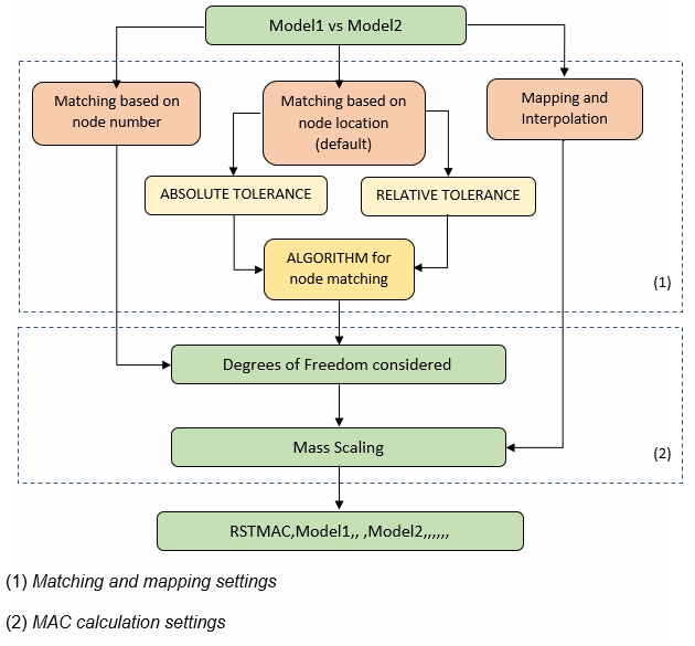
To perform all of these steps and improve the RSTMAC command results, different options are available on the MACOPT command. These options can be combined, as shown in Figure 7.20: An Overview of MACOPT Command Options.
All of the steps for MAC based calculations are detailed
below using two models of a simply supported beam. Model 1,
tsolid, is a solid element mesh. Model 2,
tbeam, is a beam element mesh.
All of the first ten eigensolutions are compared, and a full printout is
requested (KeyPrint = 2 on the
RSTMAC command).
The input is:
rstmac, tsolid,1,all, tbeam,1,all,,,, 2
The output is:
   ******************** MATCHED NODES ********************
      Node in             Node in             Distance
      tsolid.rst          tbeam.rst
         33                   1              0.0000E+00
        521                   2              0.0000E+00
        526                   4              0.0000E+00
        531                   6              0.2220E-15
        536                   8              0.4441E-15
        541                  10              0.8882E-15
        546                  12              0.1776E-14
        551                  14              0.2665E-14
        556                  16              0.3553E-14
       5000                  50              0.0000E+00
Any pair of nodes with a distance smaller than the tolerance
specified (Option = ABSTOLN and/or RELTOLN on
MACOPT) is considered matched. If there
are no pair of nodes within the tolerance specified , the node matching is
failing and the MAC calculations will not be performed.
For specifying the tolerance on the MACOPT command, you
can choose either an absolute tolerance applied to the distance between
nodes (ABSTOLN) or a relative tolerance which is
a fraction of the minimum element dimension
(RETOLN). The absolute tolerance value
specified must be smaller than the element size to obtain relevant matched
pairs.
By default, to get matched pairs, the node matching algorithm finds the first node with distance below the tolerance. If you specify the option KEYALGONOD = YES on MACOPT, then the node matching algorithm finds the nearest node with distance below the tolerance.
Only the matched nodes will contribute to the MAC calculations.
If you want to match a set of selected nodes only, you may do one of the following:
First, the database corresponding to tsolid
must be resumed.
When comparing the nodal solutions of cyclic symmetric structures, the database must be saved AFTER the solution is finished. The same applies when comparing solutions obtained with the linear perturbation procedures, because the node coordinates are updated with the base analysis displacements during the solution.
The input is:
macopt, NODMAP,yes
rstmac, tsolid,1,all, tbeam,1,all,,,, 2
The output is:
 ******************** MAPPED NODES ********************
              Node in             Element in
              tbeam.rst           tsolid.rst
                  1                    1
                  2                   40
                  3                    3
                  4                    5
                  5                    8
                  6                   10
                  7                   13
                  8                   15
                  9                   18
                 10                   20
                 11                   23
                 12                   25
                 13                   28
                 14                   30
                 15                   33
                 16                   35
                 17                   38
Only the mapped nodes will contribute to the MAC calculations.
Nodes that are coincident may lead to erroneous interpolation. For example, this can occur in the case of spring/mass systems attached to solid elements.
If nodes and/or elements are selected (NSEL and/or ESEL, respectively), the results of the mapping and/or the interpolation show differences. To perform the MAC calculation on a part of the model, you can use the ESEL command. For a cyclic analysis where the MSUP option is not activated (CYCOPT,MSUP,NO), select the elements of both the base sector and the duplicate sector. For a cyclic analysis where the MSUP option is activated (CYCOPT,MSUP,YES) select the elements of the base sector only. All selected element nodes must also be selected (NSLE).
Issue the OUTRES command only when generating the
second results file
(File2). If the OUTRES
command is issued to reduce the solution data written to the first results
file (File1), the interpolation may be incorrect.
(The problem can occur when an element does not have all of its nodes in the
results file, for example.) This option is not supported when comparing
cyclic symmetric structure results.
Model 1, tbeamx, is a beam element mesh along
X direction. Model 2, tbeamy, is a beam element
mesh along Y direction with the same node numbering as
tbeamx.
The input is:
macopt,NUMMATCH,yes
rstmac, tbeamx,1,all, tbeamy,1,all,,,, 2
The output is:
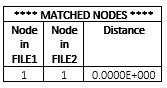
 ******************** MATCHED NODES ********************
      Node in             Node in              Distance
      FILE1               FILE2
            1                   1             0.0000E+000
            2                   2             0.1414E+001
            3                   3             0.1414E+000
            4                   4             0.2828E+000
            5                   5             0.4243E+000
            6                   6             0.5657E+000
            7                   7             0.7071E+000
            8                   8             0.8485E+000
            9                   9             0.9899E+000
           10                  10             0.1131E+001
           11                  11             0.1273E+001
Any pair of nodes with the same number is considered matched. If there are no matched node pairs, the RSTMAC fails, and the MAC calculations will not be performed.
Only the matched nodes will contribute to the MAC calculations.
A set of selected nodes can be studied using the component name
(Cname) on the RSTMAC
command.
The MAC output for interpolated solutions (mapped nodes) is:
   ****** Modal Assurance Criterion (MAC) VALUES ******
                    Solutions are real
    Rows:     10 substeps in load step  1 interpolated from file tsolid.rst
    Columns:  10 substeps in load step  1 from file tbeam.rst

           1       2       3       4       5       6       7       8       9      10
    1   1.000   0.000   0.000   0.000   0.000   0.000   0.000   0.000   0.000   0.000
    2   0.000   1.000   0.000   0.000   0.000   0.000   0.000   0.000   0.000   0.000
    3   0.000   0.000   1.000   0.000   0.000   0.000   0.000   0.000   0.000   0.000
    4   0.000   0.000   0.000   1.000   0.000   0.000   0.000   0.000   0.000   0.000
    5   0.000   0.000   0.000   0.000   1.000   0.000   0.000   0.000   0.000   0.000
    6   0.000   0.000   0.000   0.000   0.000   1.000   0.000   0.000   0.000   0.000
    7   0.000   0.000   0.000   0.000   0.000   0.000   1.000   0.000   0.000   0.000
    8   0.000   0.000   0.000   0.000   0.000   0.000   0.000   1.000   0.000   0.000
    9   0.000   0.000   0.000   0.000   0.000   0.000   0.000   0.000   1.000   0.000
   10   0.000   0.000   0.000   0.000   0.000   0.000   0.000   0.000   0.000   1.000
The modal assurance criterion values can be retrieved as parameters
(*GET with Entity =
RSTMAC).
The modes obtained after a modal analysis of a cyclic symmetric structure are repeated when the harmonic index is not equal to zero and not equal to the number of sectors divided by 2 (for an even number of sectors). In this case, the MAC values table is merged to allow the solutions matching. This merging consists of summing and averaging the MAC values of the repeated frequencies.
The MAC table and the compressed MAC table for cyclic symmetry are as follows:
   ****** Modal Assurance Criterion (MAC) VALUES ******
                    Solutions are real
    Rows:      6 substeps in load step  2 from FILE1
    Columns:  10 substeps in load step  2 from FILE2

           1       2       3       4       5       6       7       8       9      10
    1   0.998   0.002   0.017   0.132   0.000   0.004   0.000   0.000   0.001   0.008
    2   0.002   0.998   0.132   0.017   0.004   0.000   0.000   0.000   0.008   0.001
    3   0.000   0.000   0.013   0.840   0.001   0.346   0.000   0.000   0.000   0.103
    4   0.000   0.000   0.840   0.013   0.346   0.001   0.000   0.000   0.103   0.000
    5   0.000   0.000   0.000   0.000   0.000   0.000   0.466   0.531   0.000   0.000
    6   0.000   0.000   0.000   0.000   0.000   0.000   0.531   0.466   0.000   0.000

   ***** Modal Assurance Criterion (MAC) VALUES (compressed table for CYCLIC) *****
                    Solutions are real
    Rows:      3 substeps in load step  2 from FILE1
    Columns:   5 substeps in load step  2 from FILE2

           1       3       5       7       9
    1   1.000   0.150   0.004   0.000   0.009
    3   0.000   0.853   0.347   0.000   0.103
    5   0.000   0.000   0.000   0.997   0.000
The MAC values and the merged values from the
compressed MAC table can be extracted using *GET command
(*GET, Par, RSTMAC,
N, MAC / MACCYC,
M).
MAC per node pair (Option = NMAC on
MACOPT) is computed for matched node pairs for which
a solution is available in the results file or .unv
file. Node pairs for which MAC is below the minimum acceptable value
specified (MacLim on the
RSTMAC command) will be flagged (*). Pairs of nodes
for which all degrees of freedom are zero are flagged differently
(**).
The MAC per node pair output is as follows
(MacLim = 0.9):
******** Modal Assurance Criterion per node pair ********
            Substep l in load step 1 from FILE1
            Substep l in load step 1 from FILE2
    Node in               Node in                 Nodal MAC
    FILE1                 FILE2
          1                     1                    0.000 **
          2                     2                    1.000
          3                     3                    1.000
          4                     4                    1.000
          5                     5                    1.000
          6                     6                    0.752 *
          7                     7                    1.000
          8                     8                    1.000
          9                     9                    1.000
         10                    10                    1.000
         11                    11                    1.000
In the example above, the first node pair has both nodes fixed, while the
6th pair of nodes has a MAC below the minimum acceptable value specified
(MacLim on the RSTMAC
command).
The Matched Solutions output for interpolated solutions (mapped nodes) is as follows:
   ********************************** MATCHED SOLUTIONS **********************************
    Substep in         Substep in           MAC value       Frequency          Frequency
      tsolid.rst          tbeam.rst                       difference (Hz)       error (%)
    (interpolated)
          1                   1               1.000          0.10E-01            0.2
          2                   2               1.000         -0.47E-02            0.1
          3                   3               1.000          0.26E-01            0.2
          4                   4               1.000          0.27E-01            0.1
          5                   5               1.000          0.40E-01            0.1
          6                   6               1.000          0.13E+00            0.2
          7                   7               1.000          0.11E+00            0.2
          8                   8               1.000          0.82E-01            0.1
          9                   9               1.000         -0.12E+00            0.1
         10                  10               1.000         -0.96E+00            0.6
If no pair of solutions has a MAC value greater than the minimum
acceptable value specified (MacLim on the
RSTMAC command), the matching of the solutions is
failing. The default limit is set to 0.9.
The node matching procedure is the same as described above in the MAC procedure (Matching the Nodes of Model 1 and Model 2 Based on Node Location and Matching the Nodes of Model 1 and Model 2 Based on Their Node Numbers).
The supported criteria for FRF correlation are the cross signature assurance criterion (CSAC) and the cross signature scale factor (CSF) (see POST1 – Frequency response function correlation in the Theory Reference for more details).
Depending on the FRF option on MACOPT command, CSAC or CSF or both are computed for each Substep of the frequency domain. CSAC is used to quantify the shape correlation level between the FE generated and measured FRFs at each frequency and is sensitive to changes in mass and stiffness. CSF is used to quantify the amplitude difference between the FE generated and measured FRFs at each frequency and is sensitive to changes in damping.
Note that FRF correlation is only supported for the comparison of an
.rst and a.unv file. The
.rst file must be issued from a harmonic analysis
where a unit single point excitation was applied. If the frequency domains
in the .rst file solution and .unv
file measurements are not the same, only the overlap of the two domains is
considered. If the substeps of the two files do not match, the FE generated
solution in the .rst file is interpolated to match the
substeps of the experimental data (.unv file). The
interpolation of the .rst file results may degrade the
quality of FRF correlation, especially close to the natural frequencies.
Hence, clustering frequency solutions about natural frequencies may improve
the results (FREQARR on the
HARFRQ command or Clust on
the HROUT command).
The FRF correlation results are presented in a table, and substeps for
which CSAC or CSF are below the minimum acceptable value specified
(MacLim on the RSTMAC
command) are flagged (*).
The output is as follows (MacLim = 0.9):
****** Frequency Response Function correlation ******
          Solutions are complex
          Number of substeps:   10

          Frequency:    CSAC        CSF
            55.000      1.000      1.000
            60.000      1.000      1.000
            65.000      1.000      1.000
            70.000      1.000      1.000
            75.000      1.000      1.000
            80.000      1.000      1.000
            85.000      1.000      1.000
            90.000      1.000      1.000
            95.000      1.000      1.000
           100.000      1.000      0.851 *
In the example above, the last Substep (Frequency = 100Hz) has a CSF below
the minimum acceptable value specified (MacLim on
the RSTMAC command).
The Universal Format file records supported are the following.
Dataset Number 2420: Coordinate system
Dataset Number 15 or 2411: Nodes
Dataset Number 55: Data at Nodes
Record 6
Field 1: Model Type = 1 (Structural)
Field 2: Analysis Type = 3 (Complex eigenvalue first order) or Analysis Type = 2 (Normal Mode)
Field 3: Data Characteristic = 2 (3 DOF) or 3 (6 DOF)
Field 4: Specific Data Type = 8 (Displacement) or 12 (Acceleration)
Field 5: Data Type = 2 (Real) or 5 (Complex)
Dataset Number 58: Function at Nodal DOF
Record 6
Field 1: Function Type = 4
Field 4: Load Case Identification Number 0 – Single Point Excitation
Record 8 - Abscissa Data Characteristics
Field 1: Specific Data Type = 18 (Frequency)
Record 9 - Ordinate (or ordinate numerator) Data Characteristics
Field 1: Specific Data Type = 8 (Displacement) or 12 (Acceleration for CSAC computation)
Record 10 – Ordinate Denominator Data Characteristics
Field 1: Specific Data Type = 13 (excitation force)
The modal assurance criterion and the cross-signature assurance criterion are normalized quantities. Multiplying one solution vector by a constant does not modify the end result. As a consequence, because the modal acceleration is equal to the modal displacement multiplied by the frequency squared, a modal displacement result on the results file can be compared to a modal acceleration vector on the .unv file.
The coordinate system transformation (Option =
UNVTRAN on MACOPT ) is based on Dataset Number 2420 and used
to transform the solution vector from the local to the global coordinate system.
Only Cartesian coordinate systems are supported,
and this option is only supported for MAC computation.
To print out the Universal Format file records, you can
use the UNVDEBUG key on MACOPT. All information is listed on
File2_unv.txt.
The following example presents some MACOPT command options and the corresponding RSTMAC results. The studied models are two slender plates clamped at one end and modeled using different element types (BEAM189 vs SHELL181), as shown in Figure 7.21: SHELL181 Model vs BEAM189 Model.
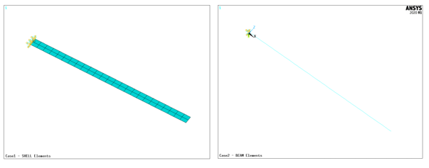
/com,
/com, ----- > Case1 – SHELL elements
/com,
/filname,case1
pi = acos(-1)

! geometry & Material
! ---------------------------
L = 1      ! beam length
b = 0.05  ! X-section breadth
h = 0.0025  ! X-section height
E  = 2.1e11
nu = 0.3
rho = 7800

parsav,,geom,parm

/prep7

! element type and material prop.
! -----------------------------------------
et,1,181
sectype,1,shell
secdata,h

mp,ex,1,E
mp,prxy,1,nu
mp,dens,1,rho

! create geometry
! ---------------------
local,11,0 ,0,0,0 ,0,90,0
wpcsys,11
blc4,0,-b/2,L,b
csys,0

! meshing
! -----------
lsel,s,loc,x,L/2
lesize,all,,, 50

lsel,s,loc,z,0
lesize,all,,, 4

allsel
amesh,all

! boundary conditions
! --------------------------
nsel,s,loc,x,0
d,all,all
allsel
finish

/solu
antype,modal
modopt,lanb,8,,,
mxpand,8
solve
finish
save

/post1
set,list
finish
/clear,nostart

/filname,case2
parres,,geom,parm

/com,
/com, ----- > Case2 – BEAM elements
/com,

/PREP7

! element type and material prop.
! -----------------------------------------
et,1,189
sectype,1,beam,rect
secdata,h,b

mp,ex,1,E
mp,prxy,1,nu
mp,dens,1,rho

! Geometry & Meshing
! ----------------------------
k,1,0,0,0.01
k,2,L,0,0.01
l,1,2

Nelt = 30
lesize,all,,,Nelt
lmesh,all

! boundary conditions
! --------------------------
nsel,s,loc,x,0
d,all,all
allsel
/eshape,1
eplot
FINISH

! Modal analysis
! --------------------
/solu
antype,modal
modopt,lanb,8,,,
mxpand,8
solve
finish

/POST1
set,list
FINISH
/clear,nostart

resume,case1,db
/com,_________________________________________________
/com,
/com,  			MAC CALCULATION
/com,_________________________________________________
/com,

/post1
/com, _____________________________________________________
/com,
/com, ---------> Case 1  Node matching based on node location (DEFAULT)
/com  ------>  Using an absolute tolerance (0.005)
/com,_____________________________________________________
MACOPT,ABSTOLN,0.005
rstmac,case1.rst,1,all,case2.rst,1,all,,0.70,,1

/com, ______________________________________________________
/com,
/com, ---------> Case 2  Node matching based on node location (DEFAULT)
/com ------> Using a higher tolerance (0.02)
/com,______________________________________________________
MACOPT,ABSTOLT,0.02
rstmac,case1.rst,1,all,case2.rst,1,all,,0.70,,1

/com, _______________________________________
/com,
/com, ---------> Case 3  Node mapping
/com,_______________________________________
MACOPT,NODMAP,yes
rstmac,case1.rst,1,all,case2.rst,1,all,,0.70,,1

finish
The table below summarizes the results for the three cases. Although the MAC values depend on the method used to match or map the nodes, they are all very close to 1.0. A high number of matched nodes does not necessarily improve the MAC value. The tolerance should be chosen carefully to match relevant nodes.
Table 7.5: MACOPT Commands and Results of RSTMAC Command for All Cases
| Case 1 | Case 2 | Case 3 | ||
|---|---|---|---|---|
| Matching / mapping method | Matching based on node location | Mapping | ||
| MACOPT command |
MACOPT,ABSTOLN,0.005 |
MACOPT,ABSTOLN,0.02 |
MACOPT,NODMAP,yes | |
| Resulting matched / mapped nodes | *** NOTE *** Node matching in RSTMAC command succeeded. 31 pairs of nodes are within the tolerance (.005). | *** NOTE *** Node matching in RSTMAC command succeeded. 61 pairs of nodes are within the tolerance (.02). | *** NOTE *** Node mapping in RSTMAC command succeeded. 61 nodes are mapped. | |
| Substep in FILE1 | Substep in FILE2 | Calculated MAC values | ||
| 1 | 1 | 1.000 | 1.000 | 1.000 |
| 2 | 2 | 1.000 | 0.996 | 1.000 |
| 3 | 3 | 0.999 | 0.990 | 1.000 |
| 4 | 4 | 0.999 | 0.998 | 1.000 |
| 5 | 5 | 0.999 | 0.981 | 1.000 |
| 7 | 7 | 0.998 | 0.969 | 1.000 |
| 8 | 8 | 0.997 | 0.956 | 1.000 |
The example shown here demonstrates how RSTMAC results can be improved when relevant degrees of freedom and the appropriate matching method are chosen.
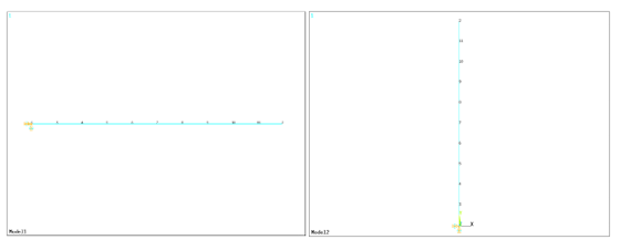
Two models of simply supported beam are compared in this example. The first beam is meshed along X direction, and the second one is meshed along Y direction, as shown in Figure 7.22: Two Simply Supported Beams..
/filname,Model1
/PREP7
! parameters
! ---------------

! geometry
        Lb = 1 			! length of beam
        bb = 0.01 		! X-section breadth
        hb = 0.02 		! X-section height
! material
        E   = 1e11
        nu  = 0.3
        rho = 8000
! mesh
        Ndiv = 10

! element types & material
! ----------------------------------
et,1,188 ! beam element
sectype,1,beam,rect
secdata,bb,hb

mp,ex,1,E
mp,prxy,1,nu
mp,dens,1,rho

! geometry & meshing
! ---------------------------
k,1 ,0 ,0,0
k,2 ,Lb,0,0
l,1,2
allsel

lesize,all,,,Ndiv
secnum,1
lmesh,all

! boundary conditions
! ---------------------------
nsel,s,loc,x,0
d,all,all

allsel
FINISH

/SOLU
antype,modal
modopt,lanb,8
allsel
solve
FINISH

/POST1
set,list
FINISH
/clear,nostart
/filname,Model2
/PREP7

! parameters
! ----------------

! geometry
        Lb = 1    ! length of beam
        bb = 0.01 ! X-section breadth
        hb = 0.02 ! X-section height
! material
        E   = 1e11
        nu  = 0.3
        rho = 8000
! mesh
        Ndiv = 10

! element types & material
! --------------------------------
et,1,188 ! beam element
sectype,1,beam,rect
secdata,bb,hb

mp,ex,1,E
mp,prxy,1,nu
mp,dens,1,rho

! geometry & meshing
! ---------------------------
k,1 ,0,0 ,0
k,2 ,0,Lb,0
l,1,2
allsel

lesize,all,,,Ndiv
secnum,1
lmesh,all

! boundary conditions
! ---------------------------
nsel,s,loc,y,0
d,all,all
allsel
FINISH

/SOLU
antype,modal
modopt,lanb,8
allsel
solve
FINISH

/POST1
set,list
FINISH

/com ==========================================================================
/com                             MAC COMPARISON
/com ==========================================================================
/clear,nostart

/POST1
/out
/com --------------------------------------------------------------------------
/com    Case 1  default matching based on node location
/com        --> One node should be matching
/com --------------------------------------------------------------------------

rstmac,Model1.rst,,,Model2.rst,,,,,,2

/com --------------------------------------------------------------------------
/com    Case 2  matching based on node number
/com        --> All nodes should be matching
/com        --> Only bending modes in Z direction should match
/com --------------------------------------------------------------------------

macopt,nummatch,1
rstmac,Model1.rst,,,Model2.rst,,,,,,2

/com --------------------------------------------------------------------------------------------------
/com    Case 3  matching based on node number & (UZ + ROTZ) dof only
/com        --> All nodes should be matching
/com        --> All modes should be matching except the 9th
/com --------------------------------------------------------------------------------------------------

macopt,nummatch,1
macopt,dof,rotz
macopt,dof,uz
rstmac,Model1.rst,,,Model2.rst,,,,,,2

FINISH
The following table summarizes the RSTMAC calculations for the three cases above. Matching based on node number is more appropriate in this case. Results can also be improved when specific degrees of freedom are compared: in this case, UZ and ROTZ.
Table 7.6: RSTMAC Command Results for All Cases
| Case 1 | Case 2 | Case 3 | |
| Matched nodes | Matching based on node location (DEFAULT)
 | Matching based
on nodes number
(MACOPT,NUMMATCH,YES)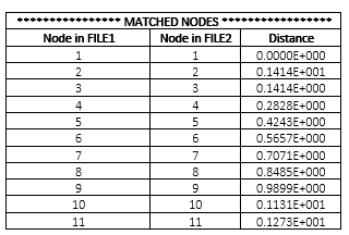 | |
| Matched solutions | *** WARNING *** No MAC value is greater than the smallest acceptable value (.9). Solutions matching in RSTMAC failed to identify pairs of solutions. | Only bending modes in Z direction matched
(All structural degrees of freedom are considered –
DEFAULT) | All modes matched (Only UZ and ROTZ
degrees of freedom are considered using
MACOPT,DOF) |