


After the desired results data are stored in the database, you can review them via graphics displays and tabular listings. You can also map the results data onto a path.
You can display the following types of graphics in POST1:
Contour displays show how a result item (such as stress, temperature, magnetic flux density, etc.) varies over the model. Four commands are available for contour displays:
The PLNSOL command produces contour lines that are continuous across the entire model. Use either for primary as well as derived solution data. Derived solution data, which are typically discontinuous from element to element, are averaged at the nodes so that continuous contour lines can be displayed.
Sample contour displays of primary data (TEMP) and derived data (TGX) are shown below.
PLNSOL,TEMP ! Primary data: degree of freedom TEMP
If PowerGraphics is enabled, you can control averaging of derived data via the AVRES command.
Any of the above allows you to specify whether or not results will be averaged at element boundaries where material and/or real constant discontinuities exist. For more information, see PowerGraphics.
Caution: If PowerGraphics is disabled, you cannot issue the AVRES command to control averaging, and the averaging operation is performed at all nodes of the selected elements without regard to the attributes of the elements connected to them. This can be inappropriate in areas of material or geometric discontinuities. When contouring derived data (which are averaged at the nodes), be sure to select elements of the same material, same thickness (for shells), same element coordinate system orientation, etc.
PLNSOL,TG,X ! Derived data: thermal gradient TGX
See the PLNSOL command description for further information.
The PLESOL command produce contour lines that are discontinuous across element boundaries. Use this type of display mainly for derived solution data. For example:
PLESOL,TG,X
The PLETAB command contours data stored in the element table. The Avglab field on the PLETAB command gives you the option of averaging the data at nodes (for continuous contours) or not averaging (the default, for having discontinuous contours). The example below assumes a layered shell (SHELL281) model and shows the difference between averaged and nonaveraged results.
ETABLE,SHEARXZ,SMISC,9     ! Interlaminar shear (ILSXZ) at bottom of layer 2
PLETAB,SHEARXZ,AVG         ! Averaged contour plot of SHEARXZ
PLETAB,SHEARXZ,NOAVG ! Nonaveraged (default) contour plot of SHEARXZ
The PLLS command displays line element results in the form of contours. The command also requires data to be stored in the element table. This type of display is commonly used for shear and moment diagrams in beam analyses.
|
Isosurface contour displays |
You can produce isosurface contour displays via the
| |
|
Averaged principal stresses |
By default, principal stresses at each node are calculated from averaged component stresses. You can reverse this operation so that principal stresses are first calculated per element, then averaged at the nodes (AVPRIN). Averaging operations should not be performed at nodal interfaces of differing materials. | |
|
Vector sum data |
These follow the same practice as the principal stresses. By default, the vector sum magnitude (square root of the sum of the squares) at each node is calculated from averaged components. You can reverse this operation (AVPRIN) so that the vector sum magnitudes are first calculated per element, then averaged at the nodes. | |
|
Shell elements or layered shell elements |
By default, results for shell or layered elements are assumed to be at the top surface of the shell or layer. You can display results at the top, middle or bottom surface (SHELL), and display the layer number for layered elements (LAYER). | |
|
von Mises equivalent strains (EQV): |
The effective Poisson's ratio used in computing these quantities can be changed (AVPRIN). Typically, the effective Poisson's ratio is set to the input Poisson's ratio for elastic equivalent strain (item and component EPEL,EQV) and to 0.5 for inelastic strains (item and component EPPL,EQV or EPCR,EQV). For total strains (item and component EPTOT,EQV), you typically use an effective Poisson's ratio between the input Poisson's ratio and 0.5. Alternatively, you can save the equivalent elastic strains (ETABLE) with the effective Poisson's ratio equal to the input Poisson's ratio and save the equivalent plastic strains in another table using 0.5 as the effective Poisson's ratio, then combine the two table entries via SADD to obtain the total equivalent strain. | |
|
Effect of /EFACET | When viewing continuous contour plots
(PLNSOL), you may notice
different plots according to the
/EFACET command argument
( /EFACET,1 -- The contour values for the intermediate locations are interpolated based on the average of the adjacent averaged corner node values. /EFACET,2 -- The midside node values are first calculated within each element, based on the average of the adjacent nonaveraged corner node values. The midside node values are then averaged together for a PLNSOL contour plot. /EFACET,4 -- The program uses shape functions to calculate results values at three subgrid points along each element edge. The subgrid values are first calculated within each element and are then averaged together for PLNSOL plots; therefore, the contour values at the midside locations will differ based on the /EFACET argument. In most cases, PLESOL contours will be the same regardless of the /EFACET arguments.
|
You can use deformed shape displays in a structural analysis to see how the structure has deformed under the applied loads. To generate a deformed shape display, issue the PLDISP command.
For example, you might issue the following PLDISP command:
PLDISP,1 ! Deformed shape superimposed over undeformed shape
You can change the displacement scaling by issuing the /DSCALE command.
When you enter POST1, all load symbols are deactivated. Load symbols remain off if you subsequently re-enter the PREP7 or SOLUTION processors. If you activate the load symbols in POST1, the resulting display shows the loads on the deformed shape.
Vector displays use arrows to show the variation of both the magnitude and direction of a vector quantity in the model. Examples of vector quantities are displacement (U), rotation (ROT), magnetic vector potential (A), magnetic flux density (B), thermal flux (TF), thermal gradient (TG), fluid velocity (V), principal stresses (S), etc.
To produce a vector display, issue the PLVECT command. For example:
PLVECT,B ! Vector display of magnetic flux density
To scale the arrow lengths, issue the /VSCALE command.
You can also create your own vector quantity by specifying two or three components on the PLVECT command.
Path plots graphs that show the variation of a quantity along a predefined path through the model. To produce a path plot, you need to perform these tasks:
For more information, see Mapping Results onto a Path.
Reaction force displays are similar to boundary condition displays and are activated via the labels RFOR or RMOM on the /PBC command. Any subsequent display (produced by commands such as NPLOT, EPLOT, or PLDISP) will include reaction force symbols at points where DOF constraints were specified. The sum of nodal forces for a DOF belonging to a constraint equation does not include the force passing through that equation.
As with reactions, you can display nodal forces via labels NFOR or NMOM on the /PBC command. These are forces exerted by an element on its node. The sum of these forces at each node is usually zero except at constrained nodes or at nodes where loads were applied.
By default in a dynamics analysis, the force (or moment) values that are printed and plotted represent the total forces (sum of the static, damping, and inertial components). The FORCE command enables you to separate the total force into individual components in all dynamics analyses except for modal analysis and spectrum analysis. In this last case, the force type is directly input on the combination command.
A charged particle trace is a graphics display that shows how a charged particle travels in an electric or magnetic field. See Creating Geometric Results Displays for more information on graphic displays and see Animation for information on particle trace animation. See the Mechanical APDL Theory Reference for simplifying assumptions on electromagnetic particle tracing.
A charged particle trace requires two commands:
The Item and
Comp fields on the PLTRAC
command enable you to see the variation of a specified item (such as electric
potential for a charged particle trace). The variation of the item is displayed
along the path trajectory as a color-contoured ribbon.
Figure 7.8: Charge Particle Trace in Electric and/or Magnetic Fields
Tracing a particle moving in a pure magnetic field might look like this:

The path of that particle moving through a pure electric field might look like this:
Plotting that same particle in the presence of both the electric and magnetic fields (with E normal to B) would then look like this:
Other useful commands are:
Three array parameters are created at the time of the particle trace: TRACPOIN, TRACDATA and TRACLABL. The parameters can be used to put the particle velocity and the elapsed time into path form.
The procedure for putting the arrays into a path named PATHNAME is:
*get,npts,PARM,TRACPOIN,DIM,x
PATH,PATHNAME,npts,9,1
PAPUT,TRACPOIN,POINTS
PAPUT,TRACDATA,TABLES
PAPUT,TRACLABL,LABELS
PRPATH,S,T_TRACE,VX_TRACE,VY_TRACE,VZ_TRACE,VS_TRACE
For charged particle traces, the variables Chrg
and Mass (input via the TRPOIN
command) have units of coulombs and kilograms, respectively, in the MKS
system.
The particle tracing algorithm could lead to an infinite loop. For
example, a charged particle trace could lead to an infinite circular loop.
To avoid infinite loops, the PLTRAC command argument
MXLOOP sets a limiting value.
Charged particle tracing can be performed after an electrostatic analysis (using only electric field), or after a magnetostatic analysis using only magnetic field or coupled magnetic and electric fields. The latter case could be done using the electric field as a body load applied either with BFE,EF command or with LDREAD,EF command.
You can map any nodal results data onto a user defined surface in POST1. You can then perform mathematical operations on these surface results to calculate meaningful quantities, including total force or average stress for a cross section, net charge inside a closed volume, fluid mass flow rate, heat flow for a cross section, and more. You can also plot contours of the mapped results.
A full complement of surface commands is provided to perform surface operations. See Surface Operations in the Command Reference.
You can define surfaces only in models containing 3D solid elements. Shells, beams and 2D element types are not supported. Surface creation will operate on selected, valid 3D solid elements only and ignore other element types if they are present in your model.
The basic steps for surface operations are as follows:
After your data is mapped on the surface, you can review the results via the graphical display and the tabular listing capabilities (SUPL, SUPR).
Additional capabilities include archiving the surface data you create to a file or an array parameter, and recalling stored surface data. The following topics relate primarily to surface definition and usage:
- 7.2.2.1. Defining the Surface
- 7.2.2.2. Mapping Results Data Onto a Surface
- 7.2.2.3. Reviewing Surface Results
- 7.2.2.4. Performing Operations on Mapped Surface Result Sets
- 7.2.2.5. Archiving and Retrieving Surface Data to a File
- 7.2.2.6. Archiving and Retrieving Surface Data to an Array Parameter
- 7.2.2.7. Deleting a Surface
Define your surface via the SUCR command. The command creates your named surface (containing no more than eight characters), according to a specified category (plane, cylinder, or sphere), at a defined refinement level.
The surfaces you create fall into three categories:
A cross section based on the current working plane
A closed surface represented by a sphere at the current working plane origin, with a user-specified radius.
A cylindrical surface centered at the working plane origin, and extending infinitely in the positive and negative Z directions
For SurfType = CPLANE,
nRefine refers to the number of points that
define the surface. If SurfType = CPLANE, and
nRefine = 0, the points reside where the cutting
plane section cuts through the element. Increasing
nRefine to 1 will subdivide each surface facet
into 4 subfacets, therefore increasing the number of points at which the results
can be interpolated. nRefine can vary between 0 and
3. Increasing nRefine can have significant effect on
memory and speed of surface operations.
/EFACET operations add to this refinement, and values
greater than 1 can amplify the effect of nRefine. An
/EFACET setting greater than 1 divides the elements into
subelements, and nRefine then refines the facets of
the subelements.
For SurfType = SPHERE, and INFC,
nRefine is the number of divisions along a
90° arc of the sphere (default is 90, Min = 10, Max = 90).
Each time you create a surface, the following predefined geometric items are calculated and stored:
GCX, GCY, GCZ -- Global Cartesian coordinates at each point on the surface.
NORMX, NORMY, NORMZ -- Components of the unit normal at each point on the surface.
DA -- Contributory area of each point.
The program uses the geometric items to perform mathematical operations with surface data; for example, DA is required to calculate surface integrals). After you create a surface, these quantities (using the predefined labels) are available for all subsequent math operations.
Issue SUPL,SurfName to display
your defined surface. A maximum of 100 surfaces can exist within one model, and
all operations (mapping results, math operations, etc.) will be carried out on
all selected surfaces. Issue the SUSEL command to change the
selected surface set.
See the SUCR command for more information of creating surfaces. When you define a cylinder (INFC), it is terminated at the geometric limits of your model. Also, any facet lying outside of those limits is discarded.
After defining a surface, issue the SUMAP command to map your data onto that surface. Nodal results data in the active results coordinate system is interpolated onto the surface and operated on as a result set. Your result sets can be made up of primary data (nodal DOF solution), derived data (stress, flux, gradients, etc.), and other results values.
Define your mapped data by providing a name for the result set, then specifying the type of data and the directional properties.
You can make the results coordinate system match the active coordinate system (used to define the path) by issuing the following pair of commands:
*GET,ACTSYS,ACTIVE,,CSYS
RSYS,ACTSYS
The first command creates a user-defined parameter named ACTSYS that holds the value defining the currently active coordinate system. The second command sets the results coordinate system to the coordinate system specified by ACTSYS.
Results mapped on to a surface do not account for discontinuities (such as material discontinuities) but are based on the currently selected set of elements. Selecting the proper set of elements is critical to valid surface operations, and improper selection can lead to failed mapping or invalid results.
To clear result sets from the selected surfaces (except GCX, GCY, GCZ, NORMX,
NORMY, NORMZ, DA), issue
SUMAP,RSetname,CLEAR. To form
additional labeled result sets by operating on existing surface result sets,
issue the SUEVAL, SUVECT or
SUCALC commands.
Issue the SUPL command to visually display your surface results, or issue SUPR to obtain a tabular listing.
For a single result set item, SUPL displays a contour plot
on the selected surfaces. You can also obtain a vector plot (such as for fluid
velocity vector) by using a special result set naming convention. If
SetName is a vector prefix (that is, if SetNameX,
SetNameY, and SetNameZ exist), the program plots the vectors on the surface as
arrows.
Example 7.3: Vector Plot
SUCREATE,SURFACE1,CPLANE       ! Create a surface called "SURFACE1"
SUMAP,VELX,V,X                 ! Map x,y,z velocities with VEL as prefix
SUMAP,VELY,V,Y
SUMAP,VELZ,V,Z
SUPLOT,SURFACE1,VEL            ! Results in a vector plot of velocities
Display of facet outlines on the surface plots is controlled by the /EDGE command, similar to other postprocessing plots.
These commands are available for mathematical operations among surface result sets:
SUCALC -- Add, multiply, divide, exponentiate and perform trigonometric operations on all selected surfaces.
SUVECT -- Calculate the cross or dot product of two result vectors on all selected surfaces.
SUEVAL -- Calculate surface integral, area weighted average, or sum of a result set on all selected surfaces. The result of this operation is an APDL scalar parameter.
You can store your surface data in a file, so that when you leave POST1, it can be retrieved later. You issue the SUSAVE command to store your data. After saving the information for your surface, issue the SURESU command to retrieve it.
You can opt to archive all defined surfaces, all selected surfaces or only a specified surface. When you retrieve surface data, it becomes the currently active surface data. Any existing surface data is cleared.
Example 7.4: Archiving and Retrieving Operations
/post1
! define spherical surface at WP origin, with a radius of 0.75 and 10 divisions per 90 degree arc
sucreate,surf1,sphere,0.75,10
wpoff,,,-2                                ! offset working plane
! define a plane surface based on the intersection of working plane
! with the currently selected elements
sucreate,surf2,cplane

susel,s,surf1           ! select surface 'surf1'
sumap,psurf1,pres   ! map pressure on surf1. Result set name "psurf1"
susel,all                  ! select all surfaces
sumap,velx,v,x      ! map VX on both surfaces. Result set name "velx"
sumap,vely,v,y      ! map VY on both surfaces. Result set name "vely"
sumap,velz,v,z      ! map VZ on both surfaces. Result set name "velz"

supr                      ! global status of current surface data
supl,surf1,sxsurf1  !  contour plot result set sxsurf1
supl,all,velx,1          ! contour plot result set velx on all surfaces. Plot in context of all elements in
model
supl,surf2,vel        ! vector plot of resultant velocity vector on surface "surf2"

suvect, vdotn,vel,dot,normal    !  dot product of velocity vector and surface normal
                                                 !  result is stored in result set "vdotn"
sueval, flowrate, vdotn, INTG         ! integrate "vdotn" over area to get apdl parameter "flow rate"
susave,all,file,surf                  ! Store defined surfaces in a file
finish
Writing surface data to an array allows you to perform APDL operations on your result sets. Issue the SUGET command to write either the interpolated results data only (default), or the results data and the geometry data to your defined parameter. The parameter is automatically dimensioned and filled with data.
An effective method for documenting analysis results (for use in reports or presentations, for example) is to produce tabular listings in POST1. Listing options are available for nodal and element solution data, reaction data, element table data, and more:
To list specified nodal solution data (primary as well as derived), issue the PRNSOL command.
Example 7.5: PRNSOL,S Listing
 PRINT S    NODAL SOLUTION PER NODE

 ***** POST1 NODAL STRESS LISTING *****

  LOAD STEP=     5  SUBSTEP=     2
   TIME=    1.0000      LOAD CASE=   0

  THE FOLLOWING X,Y,Z VALUES ARE IN GLOBAL COORDINATES

   NODE    SX          SY          SZ          SXY         SYZ         SXZ
      1   148.01     -294.54      .00000E+00 -56.256      .00000E+00  .00000E+00
      2   144.89     -294.83      .00000E+00  56.841      .00000E+00  .00000E+00
      3   241.84      73.743      .00000E+00 -46.365      .00000E+00  .00000E+00
      4   401.98     -18.212      .00000E+00 -34.299      .00000E+00  .00000E+00
      5   468.15     -27.171      .00000E+00  .48669E-01  .00000E+00  .00000E+00
      6   401.46     -18.183      .00000E+00  34.393      .00000E+00  .00000E+00
      7   239.90      73.614      .00000E+00  46.704      .00000E+00  .00000E+00
      8  -84.741     -39.533      .00000E+00  39.089      .00000E+00  .00000E+00
      9   3.2868     -227.26      .00000E+00  68.563      .00000E+00  .00000E+00
     10  -33.232     -99.614      .00000E+00  59.686      .00000E+00  .00000E+00
     11  -520.81     -251.12      .00000E+00  .65232E-01  .00000E+00  .00000E+00
     12  -160.58     -11.236      .00000E+00  40.463      .00000E+00  .00000E+00
     13  -378.55      55.443      .00000E+00  57.741      .00000E+00  .00000E+00
     14  -85.022     -39.635      .00000E+00 -39.143      .00000E+00  .00000E+00
     15  -378.87      55.460      .00000E+00 -57.637      .00000E+00  .00000E+00
     16  -160.91     -11.141      .00000E+00 -40.452      .00000E+00  .00000E+00
     17  -33.188     -99.790      .00000E+00 -59.722      .00000E+00  .00000E+00
     18   3.1090     -227.24      .00000E+00 -68.279      .00000E+00  .00000E+00
     19   41.811      51.777      .00000E+00 -66.760      .00000E+00  .00000E+00
     20  -81.004      9.3348      .00000E+00 -63.803      .00000E+00  .00000E+00
     21   117.64     -5.8500      .00000E+00 -56.351      .00000E+00  .00000E+00
     22  -128.21      30.986      .00000E+00 -68.019      .00000E+00  .00000E+00
     23   154.69     -73.136      .00000E+00  .71142E-01  .00000E+00  .00000E+00
     24  -127.64     -185.11      .00000E+00  .79422E-01  .00000E+00  .00000E+00
     25   117.22     -5.7904      .00000E+00  56.517      .00000E+00  .00000E+00
26 -128.20 31.023 .00000E+00 68.191 .00000E+00 .00000E+00
27 41.558 51.533 .00000E+00 66.997 .00000E+00 .00000E+00
28 -80.975 9.1077 .00000E+00 63.877 .00000E+00 .00000E+00MINIMUM VALUES NODE 11 2 1 18 1 1 VALUE -520.81 -294.83 .00000E+00 -68.279 .00000E+00 .00000E+00
 MAXIMUM VALUES
 NODE         5           3           1           9           1           1
 VALUE    468.15      73.743      .00000E+00  68.563      .00000E+00  .00000E+00
To list specified results for selected elements, issue the PRESOL command. To obtain line element solution printout, specify the ELEM option. The command returns all applicable element results for the selected elements.
You have several options in POST1 for listing reaction loads and applied loads. The PRRSOL command lists reactions at constrained nodes in the selected set.
In all dynamics analyses except for spectrum analyses, the FORCE command used with PRRFOR (not menu accessible) dictates which component of the reaction data is listed: total (default), static, damping, or inertia. In spectrum analyses, the force type is input on the combination command.
The PRNLD command lists the summed element nodal loads for the selected nodes, except for any zero values.
The output of summed nodal forces (PRRFOR, NFORCE, FSUM commands, etc.) containing a node that belongs to a constraint equation or part of an MPC bonded contact region (or pilot node) does not include the force redistribution due to the constraints. Issue PRRSOL, as it contains the redistribution.
Listing reaction loads and applied loads is a good way to check equilibrium. It is always good practice to check a model's equilibrium after solution. (The sum of the applied loads in a given direction should equal the sum of the reactions in that direction. If the sum of the reaction loads is not what you expect, check your loading to see if it was applied properly.)
The presence of coupling or constraint equations can induce either an actual or apparent loss of equilibrium. Actual loss of load balance can occur for poorly specified couplings or constraint equations (a usually undesirable effect). Coupled sets created by CPINTF and constraint equations created by CEINTF or CERIG will in nearly all cases maintain actual equilibrium. Other cases where you may see an apparent loss of equilibrium are: (a) 4-node shell elements where all 4 nodes do no lie in an exact flat plane, (b) elements with an elastic foundation specified, and (c) unconverged nonlinear solutions. See the Mechanical APDL Theory Reference.
The FSUM command calculates and lists the force and moment summation for the selected set of nodes.
Example 7.6: FSUM Output
 *** NOTE ***
 Summations based on final geometry and will not agree with solution
  reactions.
 ***** SUMMATION OF TOTAL FORCES AND MOMENTS IN GLOBAL COORDINATES *****
  FX  =   .1147202
  FY  =   .7857315
  FZ  =   .0000000E+00
  MX  =   .0000000E+00
  MY  =   .0000000E+00
  MZ  =   39.82639
SUMMATION POINT= .00000E+00 .00000E+00 .00000E+00
The NFORCE command provides the force and moment summation for each selected node, in addition to an overall summation.
Example 7.7: NFORCE Output
***** POST1 NODAL TOTAL FORCE SUMMATION *****
LOAD STEP= 3 SUBSTEP= 43
THE FOLLOWING X,Y,Z FORCES ARE IN GLOBAL COORDINATES
  NODE      FX         FY         FZ
     1  -.4281E-01  .4212      .0000E+00
     2   .3624E-03  .2349E-01  .0000E+00
     3   .6695E-01  .2116      .0000E+00
     4   .4522E-01  .3308E-01  .0000E+00
     5   .2705E-01  .4722E-01  .0000E+00
     6   .1458E-01  .2880E-01  .0000E+00
     7   .5507E-02  .2660E-01  .0000E+00
     8  -.2080E-02  .1055E-01  .0000E+00
     9  -.5551E-03 -.7278E-02  .0000E+00
    10   .4906E-03 -.9516E-02  .0000E+00
*** NOTE *** Summations based on final geometry and will not agree with solution reactions.
 ***** SUMMATION OF TOTAL FORCES AND MOMENTS IN GLOBAL COORDINATES *****
  FX  =   .1147202
  FY  =   .7857315
  FZ  =   .0000000E+00
  MX  =   .0000000E+00
  MY  =   .0000000E+00
  MZ  =   39.82639
SUMMATION POINT= .00000E+00 .00000E+00 .00000E+00
The SPOINT command defines the point (any point other than the origin) about which moments are summed.
To list specified data stored in the element table, issue the PRETAB command
To list the sum of each column in the element table, issue the SSUM command.
Example 7.8: PRETAB and SSUM Output
***** POST1 ELEMENT TABLE LISTING *****

   STAT    CURRENT     CURRENT     CURRENT
   ELEM    SBYTI       SBYBI       MFORYI
      1   .95478E-10 -.95478E-10 -2500.0
      2  -3750.0      3750.0     -2500.0
      3  -7500.0      7500.0     -2500.0
      4  -11250.      11250.     -2500.0
      5  -15000.      15000.     -2500.0
      6  -18750.      18750.     -2500.0
      7  -22500.      22500.     -2500.0
      8  -26250.      26250.     -2500.0
      9  -30000.      30000.     -2500.0
     10  -33750.      33750.     -2500.0
     11  -37500.      37500.      2500.0
     12  -33750.      33750.      2500.0
     13  -30000.      30000.      2500.0
     14  -26250.      26250.      2500.0
     15  -22500.      22500.      2500.0
     16  -18750.      18750.      2500.0
     17  -15000.      15000.      2500.0
     18  -11250.      11250.      2500.0
     19  -7500.0      7500.0      2500.0
     20  -3750.0      3750.0      2500.0
MINIMUM VALUES ELEM 11 1 8 VALUE -37500. -.95478E-10 -2500.0
 MAXIMUM VALUES
 ELEM         1          11          11
 VALUE    .95478E-10  37500.      2500.0
SUM ALL THE ACTIVE ENTRIES IN THE ELEMENT TABLE
 TABLE LABEL     TOTAL
 SBYTI     -375000.
 SBYBI      375000.
 MFORYI     .552063E-09
You can list other types of results via the following commands:
PRVECT -- Lists the magnitude and direction cosines of specified vector quantities for all selected elements.
PRPATH -- Calculates and then lists specified data along a predefined geometry path in the model. You must define the path and map the data onto the path; see Mapping Results onto a Path.
PRSECT --Calculates and then lists linearized stresses along a predefined path.
PRERR -- Lists the percent error in energy norm for all selected elements.
PRITER -- Lists iteration summary data.
PRENERGY -- Lists the energies of the entire model or the energies of the specified components.
By default, all tabular listings usually progress in ascending order of node numbers or element numbers. You can change this by first sorting the nodes or elements according to a specified result item. The NSORT command sorts nodes based on a specified nodal solution item, and ESORT sorts elements based on a specified item stored in the element table.
Example 7.9: Sorting Nodes
NSEL,...                ! Selects nodes
NSORT,S,X               ! Sorts nodes based on SX
PRNSOL,S,COMP           ! Lists sorted component stresses
Example 7.10: PRNSOL,S and Output After NSORT
PRINT S    NODAL SOLUTION PER NODE

  ***** POST1 NODAL STRESS LISTING *****

  LOAD STEP=     3  SUBSTEP=    43
   TIME=    6.0000      LOAD CASE=   0

  THE FOLLOWING X,Y,Z VALUES ARE IN GLOBAL COORDINATES

   NODE    SX          SY          SZ          SXY         SYZ         SXZ
    111  -.90547     -1.0339     -.96928     -.51186E-01  .00000E+00  .00000E+00
     81  -.93657     -1.1249     -1.0256     -.19898E-01  .00000E+00  .00000E+00
     51  -1.0147     -.97795     -.98530      .17839E-01  .00000E+00  .00000E+00
     41  -1.0379     -1.0677     -1.0418     -.50042E-01  .00000E+00  .00000E+00
     31  -1.0406     -.99430     -1.0110      .10425E-01  .00000E+00  .00000E+00
     11  -1.0604     -.97167     -1.0093     -.46465E-03  .00000E+00  .00000E+00
     71  -1.0613     -.95595     -1.0017      .93113E-02  .00000E+00  .00000E+00
     21  -1.0652     -.98799     -1.0267      .31703E-01  .00000E+00  .00000E+00
     61  -1.0829     -.94972     -1.0170      .22630E-03  .00000E+00  .00000E+00
    101  -1.0898     -.86700     -1.0009     -.25154E-01  .00000E+00  .00000E+00
      1  -1.1450     -1.0258     -1.0741      .69372E-01  .00000E+00  .00000E+00
MINIMUM VALUES NODE 1 81 1 111 111 111 VALUE -1.1450 -1.1249 -1.0741 -.51186E-01 .00000E+00 .00000E+00
 MAXIMUM VALUES
 NODE       111         101         111           1         111         111
 VALUE   -.90547     -.86700     -.96928      .69372E-01  .00000E+00  .00000E+00
To restore the original order of nodes or elements, issue the NUSORT and EUSORT commands.
In some situations, you may need to customize result listings to your specifications. The /STITLE command enables you to define up to four subtitles which will be displayed on output listings along with the main title. Other commands available for output customization are: /FORMAT, /HEADER, and /PAGE. They control such things as the number of significant digits, the headers that appear at the top of listings, the number of lines on a printed page, etc. These controls apply only to the PRRSOL, PRNSOL, PRESOL, PRETAB, and PRPATH commands.
One of the most powerful and useful features of POST1 is its ability to map virtually any results data onto an arbitrary path through your model. This enables you to perform many arithmetic and calculus operations along this path to calculate meaningful results: stress intensity factors and J-integrals around a crack tip, the amount of heat crossing the path, magnetic forces on an object, and so on. A useful side benefit is that you can see, in the form of a graph or a tabular listing, how a result item varies along the path.
You can define paths in models containing solid elements (2D or 3D) or shell elements.
Three general steps are necessary for reviewing results along a path:
After the data are interpolated, you can review them via graphics displays (PLPATH or PLPAGM) and tabular listings or perform mathematical operations such as addition, multiplication, integration, etc. Advanced mapping techniques to handle material discontinuities and accurate computations are offered in the PMAP command (issue this command prior to PDEF).
Other path operations you can perform include archiving paths or path data to a file or an array parameter and recalling an existing path with its data. The next few topics discuss path definition and usage.
To define a path, first define the path environment and then the individual path points. Define the path by picking nodes, by picking locations on the working plane, or by filling out a table of specific coordinate locations. Create the path by picking or by issuing the PATH and PPATH commands.
Provide the following information for the PATH command:
A path name (containing up to eight characters).
The number of path points (between 2 and 1000). If using graphical picking, the number of path points equals the number of picked points.
The number of sets of data which may be mapped to this path. (Four is the minimum; default is 30. There is no maximum.)
The number of divisions between adjacent points. (Default = 20, no maximum.)
Specify a coordinate system (
CS) for geometry interpolation (PPATH).
To see the status of path settings, issue a PATH,STATUS command.
The PATH and PPATH commands define the path geometry in the active CSYS coordinate system. If the path is a straight line or a circular arc, only the two end nodes are required (unless you want highly accurate interpolation, which may require more path points or divisions).
If necessary, issue the CSCIR command to move the coordinate singularity point before defining the path.
To display the path that you have defined, first interpolate data along the path, then issue the /PBC,PATH,1 command, followed by the NPLOT or EPLOT command.
The program displays the path as a series of straight line segments. The path shown here was defined in a cylindrical coordinate system:
A maximum of 100 paths can exist within one model. However, only one path at a
time can be the current path. To change the current path, choose the
PATH,NAME command. Do not
specify any other arguments on the PATH command. The named
path will become the new current path.
The path must already be defined. Issue the PDEF and PVECT commands to interpolate data along the path.
The PDEF command enables you to interpolate virtually any results data along the path in the active results coordinate system: primary data (nodal DOF solution), derived data (stresses, fluxes, gradients, etc.), element table data, and so on. The rest of this discussion (and in other documentation) refers to an interpolated item as a path item. For example, to interpolate thermal flux in the X direction along a path, the command would be as follows:
PDEF,XFLUX,TF,X
The XFLUX value is an arbitrary user-defined name assigned to the path item. TF and X together identify the item as the thermal flux in the X direction.
You can make the results coordinate system match the active coordinate system (used to define the path) by issuing the following pair of commands:
*GET,ACTSYS,ACTIVE,,CSYS
RSYS,ACTSYS
The first command creates a user-defined parameter (ACTSYS) that holds the value defining the currently active coordinate system. The second command sets the results coordinate system to the coordinate system specified by ACTSYS.
POST1 uses {nDiv(nPts-1) + 1} interpolation points to map data onto the path
(where nPts is the number of points on the
path and nDiv is the number of path divisions
between points (PATH)). When you create the first path item,
the program automatically interpolates the following additional geometry items:
XG, YG, ZG, and S. The first three are the global Cartesian coordinates of the
interpolation points and S is the path length from the starting node. These
items are useful when performing mathematical operations with path items (for
instance, S is required to calculate line integrals). To accurately map data
across material discontinuities, use the DISCON = MAT
option on the PMAP command.
To clear path items from the path (except XG, YG, ZG, and S), issue PDEF,CLEAR. To form additional labeled path items by operating on existing path items, issue the PCALC command.
The PVECT command defines the normal, tangent, or position vectors along the path. A Cartesian coordinate system must be active for this command. For example, the command shown below defines a unit vector tangent to the path at each interpolation point.
PVECT,TANG,TTX,TTY,TTZ
TTX, TTY, and TTZ are user-defined names assigned to the X, Y, and Z components of the vector. You can use these vector quantities for fracture mechanics J-integral calculations, dot and cross product operations, etc. For accurate mapping of normal and tangent vectors, use the ACCURATE option on the PMAP command. Issue the PMAP command prior to mapping data.
To obtain a graph of specified path items versus path distance, issue the PLPATH command.
To get a tabular listing of specified path items, issue the PRPATH command.
You can control the path distance range (the abscissa) for PLPATH and PRPATH via the PRANGE command. Path-defined variables can also be used in place of the path distance for the abscissa item in the path display.
To calculate and review linearized stresses along a path defined by the first two nodes on the PPATH command, you can issue either the PLSECT or PRSECT command. Typically, you use them in pressure vessel applications to separate stresses into individual components: membrane, membrane plus bending, etc. The path is defined in the active display coordinate system.
You can display a path data item as a color area contour display along the path geometry. The contour display offset from the path may be scaled for clarity. To produce such a display, issue the PLPAGM command.
If you wish to retain path data when you leave POST1, you must store it in a file or an array parameter so that you can retrieve it later. Select a path or multiple paths (PSEL), then write the current path data to a file (PASAVE).
You can then retrieve path information from the saved file and store the data as the currently active path data (PARESU).
You can archive or fetch only the path data (data mapped to path (PDEF) or the path points (defined via PPATH). When you retrieve path data, it becomes the currently active path data (existing active path data is replaced). If you issue PARESU and have multiple paths, the first path from the list becomes the currently active path.
Example 7.11: Archiving and Retrieving Path Data to a File
/post1
path,radial,2,30,35     ! Define path name, No. points, No. sets, No. divisions
ppath,1,,.2             ! Define path by location
ppath,2,,.6
pmap,,mat               ! Map at material discontinuities
pdef,sx,s,x             ! Interpret radial stress
pdef,sz,s,z             ! Interpret hoop stress
plpath,sx,sz            ! Plot stresses
pasave                  ! Store defined paths in a file
finish
/post1
paresu                  ! retrieve path data from file
plpagm,sx,,node         ! plot radial stresses on the path
finish
Writing path data to an array is useful if you want to map a charged particle trace onto a path (PLTRAC). If you wish to retain path data in an array parameter, issue the PAGET command to write current path data to an array variable.
To retrieve path information from an array variable and store the data as the
currently active path data, issue a PAPUT,
PARRAY, POPT
command.
You can archive or fetch only the path data (data mapped to path using
PDEF) or the path points (defined via
PPATH). The setting for the POPT
argument on PAGET and PAPUT determines
what is stored or retrieved. You must retrieve path points prior to retrieving
path data and labels. When you retrieve path data, it becomes the currently
active path data (existing active path data is replaced).
Example 7.12: Archiving and Retrieving Path Data to an Array Parameter
Sample input and output are shown below.
/post1
path,radial,2,30,35     ! Define path name, No. points, No. sets, No. divisions
ppath,1,,.2             ! Define path by location
ppath,2,,.6
pmap,,mat               ! Map at material discontinuities
pdef,sx,s,x             ! Interpret radial stress
pdef,sz,s,z             ! Interpret hoop stress
plpath,sx,sz            ! Plot stresses
paget,radpts,points     ! Archive path points in array "radpts"
paget,raddat,table      ! Archive path data in array "raddat"
paget,radlab,label      ! Archive path labels in array "radlab"
finish
/post1
*get,npts,parm,radpts,dim,x  ! Retrieve number of points from array "radpts"
*get,ndat,parm,raddat,dim,x  ! Retrieve number of data points from array "raddat"
*get,nset,parm,radlab,dim,x  ! Retrieve number of data labels form array "radlab"
ndiv=(ndat-1)/(npts-1)       ! Calculate number of divisions
path,radial,npts,ns1,ndiv    ! Create path "radial" with number of sets ns1>nset
paput,radpts,points          ! Retrieve path points
paput,raddat,table           ! Retrieve path data
paput,radlab,labels          ! Retrieve path labels
plpagm,sx,,node              ! Plot radial stresses on the path
finish
One of the main concerns in a finite element analysis is the adequacy of the finite element mesh. Is the mesh fine enough for good results? If not, what portion of the model should be remeshed? You can get answers to such questions with the error-estimation technique, which estimates the amount of solution error due specifically to mesh discretization. This technique is available only for linear structural and linear/nonlinear thermal analyses using 2D or 3D solid elements or shell elements.
In the postprocessor, the program calculates an energy error for each element in the model. The energy error is similar in concept to the strain energy. The structural energy error (labeled SERR) is a measure of the discontinuity of the stress field from element to element, and the thermal energy error (TERR) is a measure of the discontinuity of the heat flux from element to element. Using SERR and TERR, the program calculates a percent error in energy norm (SEPC for structural percent error, TEPC for thermal percent error).
Error estimation is based on stiffness and conductivity matrices that are evaluated at the reference temperatures (TREF). Error estimates, therefore, can be incorrect for elements with temperature-dependent material properties if those elements are at a temperature that is significantly different than TREF.
In many cases, you can significantly increase program speed by suppressing error estimation. This improved performance is most evident when error estimation is turned off in a thermal analysis. Therefore, you may want to use error estimation only when needed, such as when you wish to determine if your mesh is adequate for good results.
You may turn error estimation off issuing ERNORM,OFF. By default, error estimation is active. Since the value set by the ERNORM command is not saved on Jobname.db, you will need to reissue ERNORM,OFF if you wish to again deactivate error estimation after resuming an analysis .
In POST1 then, you can list SEPC and TEPC for all selected elements via the PRERR command. The value of SEPC or TEPC indicates the relative error due to a particular mesh discretization. To find out where you should refine the mesh, simply produce a contour display of SERR or TERR and look for high-error regions.
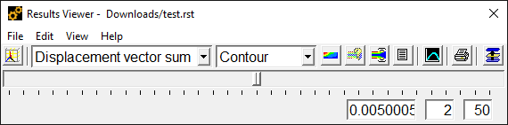
The Results Viewer is a compact toolbar for viewing your analysis results. Selecting the Results Viewer disables much of the standard GUI functionality. Many of these operations are not available because of PowerGraphics limitations. However, a good deal of the POST1 functionality is contained in the Result Viewer menu structure, and in the right and middle mouse button context sensitive menus that are accessible when you use the Results Viewer.
You can use the Results Viewer to access any data stored in a valid results file (such as *.rst, *.rth, and *.rmg). Because the viewer can access results data without loading the entire database file, it is an ideal location from which to compare data from many different analyses.
Even if you have loaded other results files, you can return to your original analysis. You can reload the original results file from the current analysis before closing the Results Viewer.
The Results Viewer has three primary control areas:
The Main Menu is located along the top of the Results Viewer and provides access to the File, Edit, View and Help menus. The following functions can be accessed from each of these headings.
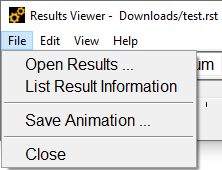
- File --
- Open Results --
Open any results file from any location on your file system.
- List Result Information --
Displays a list of all results data included in the current file.
- Save Animation --
Saves an animation file (*.anim, *.avi) to a specified location. Animations created from the Results Viewer are not written to the database.
- Close --
Closes the Results Viewer and reverts to the standard GUI.
If you have opened the results file from another analysis, return to your original file before closing the Results Viewer.
- Edit --
Select subsets of the model based on model attributes (material, element type, real ID, and element component). This selection activates the appropriate "Element Select" widget, or picking window.
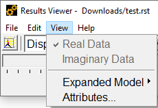
- View -
- Real Data -
Display the real data from your analysis in the graphics window. This selection is grayed out when only real data exists for your analysis.
- Imaginary Data -
Display the imaginary data for you analysis in the graphics window. This selection is grayed out when no valid imaginary data exists.
- Expanded Model -
Perform any periodic/cyclic, modal cyclic, and axisymmetric expansions available via the /EXPAND command.
- Attributes -
Access the attributes of your model (based on the conventions availabel via the /PNUM command.
The Results Viewer toolbar is located across the middle of the Results Viewer. You can choose the type of results data to plot and designate how the information should be plotted. You can also query results data from the graphics display, create animations, generate results listings, and plot or generate file exports of your screen contents.

- Element Plot
The first item on the toolbar is the element plot icon. This is the only model display available.
- Result Item Selector
This drop-down menu allows you to choose from the various types of data. The choices displayed may not always be available in your results file.
- Plot Type Selector
You left mouse click and hold down on this button and it produces a "fly out" that allows you to access the four types of results plots available - Nodal, Element, Vector and Trace.
- Query Results
You use the query tool to retrieve results data directly from selected areas in the graphics window. The picking menu is displayed, allowing you to select multiple items. The information is displayed only for the current view.
- Animate Results
You can create animations based on the information you have included in the results file. Because this information is created as a separate file, it is not saved within the results file. You must save the individual animations via the Results Viewer's Main Menu, Save Animation function.
- List Results
The list results button creates a text listing of all of the nodal results values for the selected sequence number and result item. You can print this data directly, or save it to a file for use in other applications.
- Image Capture
You can send the contents of the graphics window directly to a printer, capture the contents to another window that is created automatically, or port the contents to a graphics file in one of the popular formats (for example, PNG).
When you access a results file, the data is presented according to the sequential data sets of your original analysis. These data sets correspond to a specific time, load step, and substep of your analysis. Use the following controls to access these different result sets.
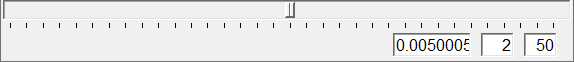
- The Data Sequence Slider Bar
The slider bar directly under the Results Viewer Toolbar corresponds to the individual data sequences that are available for the current results file. Each tick mark along the slider represents a data set. The data sequence number is displayed in the text box at the far right of the series of boxes below the slider. You can move to any data set either by moving the slider, or by entering the sequential number of the data set in the box.
- The Play and Stop Buttons
You use these buttons to move through the selected data sequence according to the defined load steps or substeps. The play button will step you through each of the data sets and when the final (maximum) set is reached, begin moving incrementally back down.
- Time
This text box displays the time for each data set.
- Load Step
Each individual load step number is displayed. You can enter a valid load step number here and that load step will be displayed.
- Substep
Each individual load substep number is displayed. You can enter a valid substep number here and that substep will be displayed.
- Sequence
The result sets are written sequentially to the results file during an analysis. This displays the sequence number from the results file. You also create additional sequences when you append the results file or add new loading data to your original analysis.
When you enter the Results Viewer, the remainder of the GUI is disabled, preventing conflicts between the limited data available in the Results Viewer and the functionality that can be accessed from the other GUI areas. Many of the functions needed to deal with the results data have been moved to "context sensitive" menus accessed via the right and middle mouse buttons.
The Results Viewer places your cursor in "picking mode" anytime you place the cursor in the graphics window. This allows you to select data sets and other screen operations dynamically, many times without accessing the Picking Menu. For the Results Viewer, the standard method of using the right mouse button to alternate between picking and unpicking has been moved to the middle mouse button. The middle mouse button allows you to change between picking and unpicking. You can choose the mode of picking desired (selection of points on the working plane, selection of existing entities in the selected set and selection of points on the screen). You can also access entity filters to limit those entities that can be selected. For the two-button PC mouse, the middle button functions are activated via the SHIFT-RIGHT MOUSE combination.
The right mouse button is used for context menus. These menus present choices that are applicable to the current selection. If you select "Screen Picking," you will get a legend data context menu if the cursor is over a legend item, and the graphics window context menu anywhere else.
If you select "WP Picking," and no points have been selected, you will get the legend or graphics context menus. If you have already selected points on the working plane, you will get a context menu that is applicable to the type of analysis you are performing. If you select "Entity Picking," and no entities are selected, you will get the standard Graphics and Legend context menus. If you have selected entities, you will get a context menu that is applicable to the current type of analysis.
- Graphics Window Context Menu
The following items are available from the context menu you get when you right mouse click anywhere in the graphics window except over the legend information.
- Replot -
Replots the screen and integrates any changes you have made.
- Display WP -
Toggles the Working Plane display (triad, grid, etc.) on and off.
- Erase Displays -
Toggles screen refreshes according to /ERASE - /NOERASE command functionality.
- Capture Image -
You can send the contents of the graphics window directly to a printer, capture the contents to another window that is created automatically, or port the contents to a graphics file in one of the popular formats (for example, PNG).
- Annotation -
You can choose between either static (2D), or dynamic (3D) annotations, and you can toggle your annotations on and off.
- Display Legend -
Toggles the legend display on and off
- Cursor Mode -
When the Results Viewer is selected, the option allows you to switch between modes of picking, that include: , , and .
- View -
Provides a drop-down list of view options: , , , , , , , and .
- Fit -
Fits the extents of the model in the graphics area.
- Zoom Back -
Returns to the previous zoom setting.
- Window Properties -
You can access limited legend and display property control, along with a number of viewing angle, rotational setting and magnification controls. The Legend Settings allow you to select which legend items will be displayed, and to specify their location in the graphics window. The Display Settings let you specify Hidden, Capped or Q-Slice displays, and to modify the Z-buffering options, including smoothing and directional light source functions or 3D options.
- Graphics Properties -
This selection refers to those settings which affect all windows specified in a multi-window layout (/WINDOW) along with access to the Working Plane Settings and Working Plane Offset widgets, and the Window Layout controls dialog boxes.
- Legend Area Context Menus
The legend area context menus will vary according to the location of your cursor in the legend, and the content of the legend data already being displayed. Right mouse clicking on the legend data provides control of the legend information, while clicking on the logo provides control of the date display and other miscellaneous functions. Clicking on the contour legend area provides a complete set of menus to customize your contour legend.
The legend setting and font control menus can be accessed from any of the legend context menus.
