Radiated Fields Observation Regions

To analyze the radiated fields associated with a design, define a radiation surface over which the fields will be calculated. Such a surface can be a boundary radiation surface, a geometry, or a custom radiation surface which you define as a face list. The values of the fields over this surface are used to compute the fields in the space surrounding the device. This space is typically split into two regions — the near-field region and the far-field region. The near-field region exists at less than a wave length from an energy source. The far field is where radiation occurs. See Radiated Fields for the specific equations used in HFSS for calculating the near and far field regions.

You can define a spherical surface over which to analyze the near or far fields by specifying a range and step size for phi and theta, or as Az over El or El over Az. This defines the spherical direction in which radiated fields will be evaluated. If you manually enter Phi or Theta component of a far field quantity when you using Az/El or El/Az far field definition, then the Report uses the Z axis of the Az/El or El/Az coordinate system definition as pole to calculate theta/phi component for rE. You can define a box over which to analyze near fields by specifying a coordinate system, length, width, height, and samples. You can define a rectangle over which to analyze near fields by specifying sample number for length and width. You can also draw a line along which to calculate the near fields.

You can also specify arbitrary near field sample point locations in the Global (or a specified Local) XYZ coordinate system as an external point list.

You also may need to edit the Global Material Environment in consideration of the far fields calculation.

Optionally, after defining the radiation surface, HFSS can compute antenna array radiation patterns and antenna parameters for designs that have analyzed a single array element. HFSS models the array radiation pattern by applying an "array factor" to the single element's pattern when far fields are calculated. You set up the array factor information by defining either a finite, 2D array geometry of uniformly spaced, equal-amplitude elements (a regular array) or an arbitrary array of identical elements distributed in 3D space with individual complex weights (a custom array.)

If the design contains finite arrays, you have the option to create a Source group under the Radiation folder in the Project tree. The Source Group lets you activate a subset of the virtual excitations (e.g. array[5,5]port1:2 …) instead of the physical excitations associated with the unit cell(s).

HFSS can also compute antenna parameters, such as the maximum intensity, peak directivity, peak gain, and radiation efficiency. For near-field analysis, HFSS can also compute maximum parameters, such as the maximum of the total E-field and the maximum E-field in the x-direction. For FEM-only designs, you can optionally set the Radiated Power Calculation method.

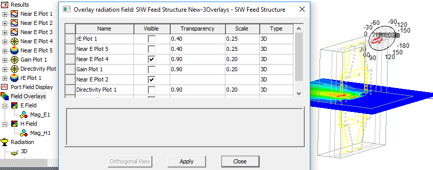
Once your have created reports, you can overlay appropriate reports on the modeler window. You can overlay multiple Results plots for radiation fields at the same time and in conjunction with other Field Overlays,and antenna parameter overlays.