Setting Field Overlay Attributes
After creating a mesh or field overlay on a surface or volume, you can modify its appearance by changing the settings in the Plot Attributes dialog box. You will modify the settings for a plot folder and all plots in that folder will use the same attributes.
- Click
 Modify Plot Attributes. Alternatively, right-click Field Overlays in the Project Manager and select Modify Attributes from the shortcut menu.
 - In the Select Plot Folder dialog box, select the plot type that you want to modify and click OK. You can also right-click the specific plot in the Project Manager and choose Modify Attributes from the shortcut menu.
- For field result overlays (not mesh plots), the available plot attributes under each tab in the dialog box are listed in the following table:
- Color map:
- Scale tab:
- Marker/Arrow
- The appearance of points (for scalar point plots).
- The appearance of arrows (for vector plots).
- Magnitude filtering (for vector plots). That is, you uncheck Map size, and specify a Min and Max Magnitude, or use a slider to set the Min threshold.
- Deformation Scale:
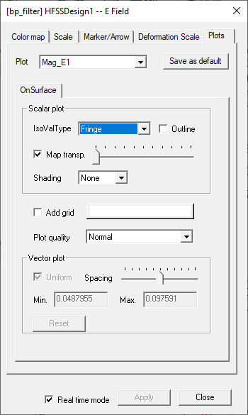
- Plots (if not vector or streamline):
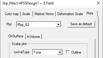
- The Plot selected. If multiple plots are available, you can select from a drop down menu. Plots can be OnSurface or InVolume. If both types are available, the dialog includes tabs for each.
- Plots can be OnSurface or InVolume. If both types are available, the dialog includes tabs for each.
- The type of isovalue display (for scalar plots.) For Line, Fringe and Tone IsoValType, Outine is enabled. For Gourad, it is disabled. The IsoValue display selection also affects InVolume, which also has other options discussed below.
- Whether to use Shading (for scalar plots), if lighting is turned on. By default, the Shading is set to None which is equivalent to "Do not use lighting."
- The transparency based on solution value.
- Whether to add a grid (that is, a mesh overlay), and to set the grid color.
- Specify the plot resolution as Coarse, Normal, Fine, or Very Fine.
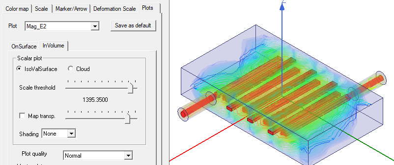
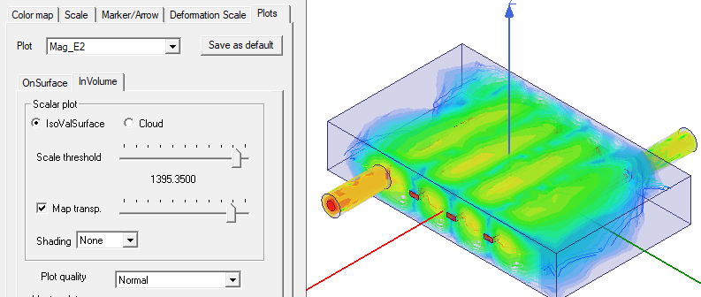
- The “Scale threshold” slider bar allows you to set a field value threshold so that iso surfaces with field value lower than the given threshold will show as translucent with given transparency specified by the slider bar below it.
- Iso surfaces with field value higher than the threshold will show as opaque. The range of the “Scale threshold” is the same as the color key range from Min to Max.
- When "Map transp." is checked, translucent iso surfaces field values map to [0.0, transparency] so lower field value map to higher transparency while higher field value to lower transparency. If it is unchecked, all translucent iso surfaces will have the same given transparency from the slider bar.
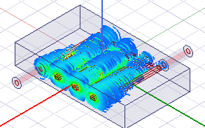
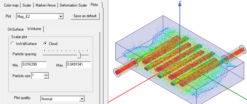
- For Cloud plots, field values are represented by points that illustrate the spatial distribution of the solution. You can use the Particle spacing slider bar to adjust the plot. The higher the solution value, the greater the cloud density. You can also specify Min and Max values (numeric values based on the active model length unit) and adjust Particle size.
- Plots (for vector plots):
- The Plot selected.
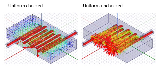
- The Min and Max spacing of arrows (for vector plots). These values are based on the model's active length unit and are only relevant when the Uniform option is selected.
- Plot quality, as Normal, Coarse, Fine, or Very Fine.
- Uniform vector spacing, based on the Spacing slider position and the Min and Max values.
- Plots (if streamline is checked):
- The Plot selected
- The Line style as solid or cylinder from drop-down menu.
- Line width, specified using a slider.
- Whether to show Marker on Streamline.
- Seeds density spacing. This affects the number of stream lines used to represent the quantity in the plot. Moving the slider to the left decreases the spacing and increases the number of stream lines. Moving the slider to the right increases the spacing and decreases the number of lines used to represent the quantity.
- Min. and Max. values represented (in Magnitude filtering settings).
- Under each tab, click Save as default if you want the tab's settings to apply to field overlay plots created after this point.
- Select Real time mode if you want the changes to take effect immediately in the view window.
- If this option is cleared, click Apply when you want to see the changes.
The Select Plot Folder dialog box appears.
A dialog box with attribute settings for the selected plot type (whether a field result or a mesh plot) appears.
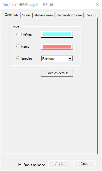
The number of colors used and how they are displayed. The field data must be available for the color key to appear.
The scale of field quantities, including the number of divisions in the scale, whether to use dB as the units, whether to use a linear or log scale, auto schall options, and plot number format.
This is for use with plots that include Stress feedback from Ansys Workbench Integration.
See Modify Plot Attributes Dialog for Stress Feedback Projects.
This affects the use of memory for animating plots. For large plots with more frames to animate, use Coarse or Normal to reduce memory requirements and improve performance. For smaller plots with few frames, if higher resolution is required, use Fine or Very Fine.
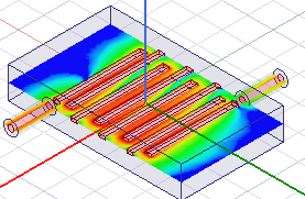
If an InVolume plot is available, and you select the tab, additional display options are available to allow visibility of internal layers and objects, particularly those with high field values. For IsoValSurface for an InVolume Scalar plot, the choices are for Scale threshold and Map transp.
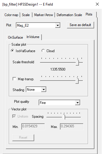
When the Map transp. slider bar is at the left most position, transparency is 0. This feature is essentially disabled, and the “Scale threshold” slider bar will be disabled. Also, high fidelity transparency should be enabled for best results.
When Uniform is not selected, a vector is rendered at every node (both corner and mid-side nodes of the elements).
The Reset button resets a good initial spacing (and thus Min, Max spacing range) without the need to recreate the field plot.