
Plotting Field Overlays
Field overlays are representations of
basic or derived field quantities on surfaces or objects for the current design variation.
You must select a geometry to create a plot. Selection of line, surface, plane, arbitrary point list, or solid object, and of scalar or vector quantities, or of the streamline option affects the display. You have more control over the display via Modify Plot Attributes.
The Plot Fields menu selections depend on the solver selected.

Electronics Desktop allows for the display of existing field overlays in the 3D Model window and Layout Editor views. You can also create plots in Layout view for specified layers and/or nets.
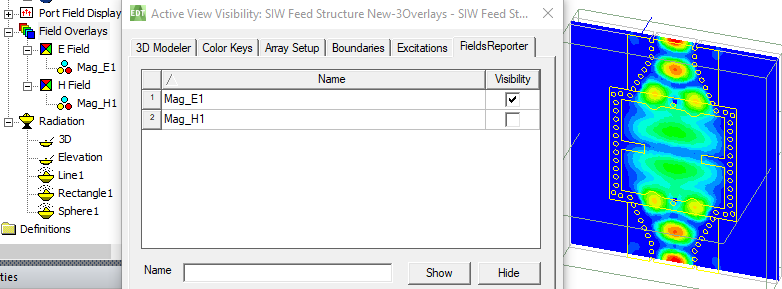
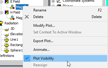
You can control the visibility of field overlays by means of the View > Visibility > Active View Visibility window, Fields Reporter tab (shown above) or by right-clicking on the Field plot in the Project Manager and checking or unchecking Plot Visibility.
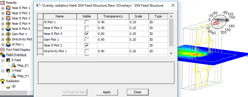
Radiation plots and antenna parameter tables available for overlay can be viewed by right-clicking Field Overlays in the History Tree, and selecting Plot Fields > Radiation Field.... This displays an Overlay radiation field window that lists each results plot available for overlay.
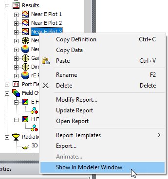
You can also control the visibility of Results plots available for the Modeler by right-clicking on the report and selecting Show in Modeler Window.
You can overlay existing 3D Polar Plots of near or far fields, near field contour plots on a near field rectangle, 2D Radiation Pattern Plots, and Monostatic or Bistatic RCS 2D plots in the model window using the HFSS 3D Layout or HFSS > Fields > Plot Fields > [Field] command, or by right-clicking on Field Overlays in the Project Manager and selecting Plot Fields > [Field]. You can also create animations of field plots.
You can overlay a 2D contour plot including Range Doppler color mapped plot to model window as a 2D overlay (which means it cannot be rotated like a geometry model). The overlay of near field on Rectangle contour plot or 2D radiation pattern plot is different. It is a 3D overlay as it can be rotated along with geometry model in 3D space.
You can also overlay tables of selected antenna parameters.
If the design includes Layout Components, the Create Field Plot dialog contains additional functionality for nets and layers.
To Plot Fields
To plot a basic field quantity
- Select a point, line, surface, plane, cutplane, or object to create the plot on or within. Your choice affects the way the fields are plotted. If you selected an object, you must check Plot on surface only to enable the Surface Smoothing button
- Click
- In the Plot Fields menu, click the field quantity you want to plot.
Available selections depend on the solved solution. For definitions of the usual quantities, see the list under Quantity command.
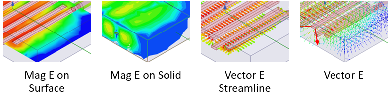
If you select a scalar field quantity, a scalar surface or volume plot will be created. If you select a vector field quantity, a vector surface or volume plot will be created. If you select a vector quantity, you will be able to specify a Streamline plot. If the quantity you want to plot is not listed, see Named Expression Library.
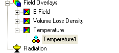
For projects with Temperature dependent materials, the HFSS 3D Layout, HFSS > Fields > Plot Fields > Other... menu selections include Temperature. For Transient projects, the menu selections show "_t" to show that they represent time dependent quantities, such as E_t, H_t, J_t, and so forth.
After you select the field quantity to plot, the Create Field Plot window appears.

The Specify Name field shows a name based on the field quantity you selected, and the Quantity list shows the field quantity selected. If the design includes Layout Components, the Create Field Plot dialog contains additional functionality for nets and layers.
- To specify a name for the plot other than the default, select Specify Name, and then type a new name in the Name field.
- Select the solution to plot from the Solution drop-down menu. Set the design variation via the Set Design Variation
window. Access this window from the Solution Data window by clicking the ellipsis button on the right of the Design Variation field, or via the
- To specify a folder other than the default in which to store the plot, select Specify Folder, and then click a folder in the Plot Folder drop-down menu, or type the name you wish to use. Plot folders are listed under Field Overlays in the Project Manager. Plot folders let you group plots with the same quantity together. All field plots under the same folder share the same color key.
- Under Intrinsic Variables, select the frequency and phase angle at which the field quantity is evaluated.
- If desired, you can select a different field quantity to plot from the Quantity list. For scalar quantities plotted on the surface of a geometry, the Surface Smoothing button is enabled. For vector quantities, the Surface Smoothing button is disabled. For details on its use, see Modifying Field Plots.
- Select the volume (region) in which the field will be plotted from the In
Volume list.
This selection enables you to limit plots to the intersection of a volume with the selected object or objects. You can select and deselect any items in the In Volume list. You can mix model objects with non-model boxes. For example, you may want to see a plot from part of two model objects by restricting the region to a non-model box overlapping those parts.
Note: Multiple selection should be used when there is a discontinuous field on a surface. If not, the field on both sides of the surface are plotted and each interferes with the other. - If you are creating a plot on a sheet object, the Adjacent checkbox allows you to create field overlays on a sheet object using data from either side of the sheet. An arrow indicates where the data is coming from. While the data is usually the same on the two sides of a sheet object, in a situation where the sheet object is assigned to be a shell element, the field may be different on its two sides. (Shell elements are an option for Layered Impedance Boundaries and Finite Conductivity Boundaries with DC conductivity and two-sided selected.) In such cases, you can visualize the field data on the side you want.
- If you selected a vector quantity, you can use the check box to select Streamline plot. Streamlines are often used to indicate magnetic flux lines, etc. in plots.
- Before creating the plot, select the starting edge (in 2D), starting surface (in 3D), or the starting points for both 2D and 3D.
- In the Creating Field Plot menu, select "In Volume: Region" which is the volume in which the streamlines will appear and is outside of the sources.
- After the plot is created, on the Attributes/Plot tab you can, you can reduce "Seeds density" to show more streamlines. If no streamlines appear, reduce this by a factor of 10 (or 100) because the default seeding was too large.
- Click Done.
The field quantity is plotted on the surfaces or within the objects you selected. The plot uses the attributes specified in the Plot Attributes window.
The new plot appears in the view window. It is listed in the specified plot folder in the project tree. Each category of plot is listed separately in the Project Manager.
If you have created a field plot on a simulation in progress, the field plot is updated after the last adaptive solution. If you want to update the field overlay before then, to view progress in the solution, select the Field icon in the Project tree that contains the field plot of interest, right-click to display the shortcut menu, and select Update Plots.
To turn off the display of the plot, right-click on the plot and select Plot Visibility from the shortcut menu. Deselect Plot Visibility to turn off the plot display.
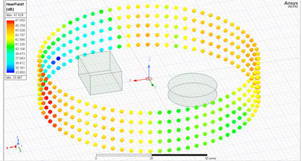
Generating a Sampled Near Field Plot
To create a Sampled Near Field Plot, based on an arbitrary Point List:
- Right-click the Field Overlays node in the Project tree, and from the shortcut menu, select Plot Sampled Near Field .... This opens the Create Near Field Plot dialog.
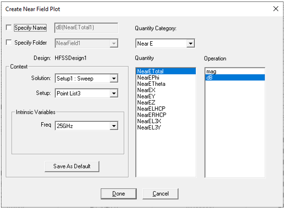
You can use the Create Near Field Plot dialog to configure which solution, quantity, and so forth.
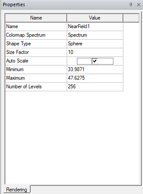
The Properties for the Plot lets you specify:
- Colormap Spectrum
- Shape Type [Point, [Point, Sphere, Box, Dot, Plus]
- Size Factor (sets size of shape marker)
- Auto Scale [On/Off] - automatically set Minimum/Maximum color scale range
- Minimum/Maximum - color scale range (linear)
- Number of Levels - sets the number of discrete color levels to use in linearly interpolating colors of shape/markers

Notes for creating Streamline plots:
See Setting Field Plot Attributes for adjusting the streamline display and Setting Fields Reporter Options for setting Streamline defaults. For exporting Streamline plots, see Exporting Field Plots.