


A transient analysis, by definition, involves loads that are a function of time. In the Mechanical application, you can perform a transient analysis on either a flexible structure or a rigid assembly. For a flexible structure, the Mechanical application can use the Ansys Mechanical APDL, Samcef, or ABAQUS solver to solve a Transient Structural analysis.
You can perform a transient structural analysis (also called time-history analysis) in the Mechanical application using the transient structural analysis that specifically uses the Ansys Mechanical APDL solver. This type of analysis is used to determine the dynamic response of a structure under the action of any general time-dependent loads. You can use it to determine the time-varying displacements, strains, stresses, and forces in a structure as it responds to any transient loads. The time scale of the loading is such that the inertia or damping effects are considered to be important. If the inertia and damping effects are not important, you might be able to use a static analysis instead.
Go to a section topic:
Points to Remember
A transient structural analysis can be either linear or nonlinear. All types of nonlinearities are allowed - large deformations, plasticity, contact, hyperelasticity, and so on. Ansys Workbench offers an additional solution method of Mode-Superposition to perform linear transient structural analysis. In the Mode-Superposition method, the transient response to a given loading condition is obtained by calculating the necessary linear combinations of the eigenvectors obtained in a modal analysis. For more details, refer to Transient Structural Analysis Using Linked Modal Analysis System section. The Mode Superposition method is not available to the Samcef or ABAQUS solver.
A transient dynamic analysis is more involved than a static analysis because it generally requires more computer resources and more of your resources, in terms of the "engineering" time involved. You can save a significant amount of these resources by doing some preliminary work to understand the physics of the problem. For example, you can:
Try to understand how nonlinearities (if you are including them) affect the structure's response by doing a static analysis first. In some cases, nonlinearities need not be included in the dynamic analysis. Including nonlinear effects can be expensive in terms of solution time.
Understand the dynamics of the problem. By doing a modal analysis, which calculates the natural frequencies and mode shapes, you can learn how the structure responds when those modes are excited. The natural frequencies are also useful for calculating the correct integration time step.
Analyze a simpler model first. A model of beams, masses, springs, and dampers can provide good insight into the problem at minimal cost. This simpler model may be all you need to determine the dynamic response of the structure.
Note: Refer to the following sections of the Mechanical APDL application documentation for a more thorough treatment of dynamic analysis capabilities:
The Transient Dynamic Analysis chapter of the Structural Analysis Guide - for a technical overview of nonlinear transient dynamics.
The Multibody Analysis Guide - for a reference that is particular to multibody motion problems. In this context, "multibody" refers to multiple rigid or flexible parts interacting in a dynamic fashion.
Although not all dynamic analysis features discussed in these manuals are directly applicable to Mechanical features, the manuals provide an excellent background on general theoretical topics.
Preparing the Analysis
As needed throughout the analysis, refer to the Steps for Using the Application section for an overview the general analysis workflow.
Define Engineering Data
Material properties can be linear or nonlinear, isotropic or orthotropic, and constant or temperature-dependent. Both Young’s modulus (and stiffness in some form) and density (or mass in some form) must be defined.
Define Part Behavior
You can define a Point Mass for this analysis type.
In a transient structural analysis, rigid parts are often used to model mechanisms that have gross motion and transfer loads between parts, but detailed stress distribution is not of interest. The output from a rigid part is the overall motion of the part plus any force transferred via that part to the rest of the structure. A "rigid" part is essentially a point mass connected to the rest of the structure via joints. Hence in a transient structural analysis the only applicable loads on a rigid part are acceleration and rotational velocity loads. You can also apply loads to a rigid part via joint loads. Rigid behavior cannot be used with the Samcef or ABAQUS solver.
If your model includes nonlinearities such as large deflection or hyperelasticity, the solution time can be significant due to the iterative solution procedure. Hence, you may want to simplify your model if possible. For example, you may be able to represent your 3D structure as a 2-D plane stress, plane strain, or axisymmetric model, or you may be able to reduce your model size through the use of symmetry or antisymmetry surfaces. Similarly, if you can omit nonlinear behavior in one or more parts of your assembly without affecting results in critical regions, it will be advantageous to do so.
Define Connections
This analysis supports Contact, Joints, and Springs.
Note: You can specify a damping coefficient property in longitudinal springs that will generate a damping force proportional to velocity.
- Samcef and ABAQUS Solvers
Only contacts, springs, and beams are supported. Joints are not supported.
Apply Mesh Controls/Preview Mesh
Provide an adequate mesh density on contact surfaces to allow contact stresses to be distributed in a smooth fashion. Likewise, provide a mesh density adequate for resolving stresses; areas where stresses or strains are of interest require a relatively fine mesh compared to that needed for displacement or nonlinearity resolution. If you want to include nonlinearities, the mesh should be able to capture the effects of the nonlinearities. For example, plasticity requires a reasonable integration point density (and therefore a fine element mesh) in areas with high plastic deformation gradients.
In a dynamic analysis, the mesh should be fine enough to be able to represent the highest mode shape of interest.
Establish Analysis Settings
For a Transient Structural analysis, the basic Analysis Settings include:
- Large Deflection
Large Deflection is typically needed for slender structures. It is typical to use large deflection if the transverse displacements in a slender structure are more than 10% of the thickness.
Small deflection and small strain analyses assume that displacements are small enough that the resulting stiffness changes are insignificant. Setting Large Deflection to On will take into account stiffness changes resulting from change in element shape and orientation due to large deflection, large rotation, and large strain. Therefore the results will be more accurate. However this effect requires an iterative solution. In addition it may also need the load to be applied in small increments. Therefore the solution may take longer to solve.
You also need to turn on large deflection if you suspect instability (buckling) in the system. Use of hyperelastic materials also requires large deflection to be turned on.
- Step Controls for Static and Transient Analyses
Step Controls enable you to control the time step size in a transient analysis. Refer to the Guidelines for Integration Step Size section for further information. In addition this control also enables you to create multiple steps. Multiple steps are useful if new loads are introduced or removed at different times in the load history, or if you want to change the analysis settings such as the time step size at some points in the time history. When the applied load has high frequency content or if nonlinearities are present, it may be necessary to use a small time step size (that is, small load increments) and perform solutions at these intermediate time points to arrive at good quality results. This group can be modified on a per step basis.
- Output Controls
Output Controls enable you to specify the time points at which results should be available for postprocessing. In a transient nonlinear analysis it may be necessary to perform many solutions at intermediate time values. However, i) you may not be interested in all the intermediate results, and ii) writing all the results can make the results file size unwieldy. This group can be modified on a per step basis except for Stress and Strain.
- Nonlinear Controls
Nonlinear Controls enable you to modify convergence criteria and other specialized solution controls. Typically you will not need to change the default values for this control. This group can be modified on a per step basis. If you are performing a nonlinear Full Transient Structural analysis, the Newton-Raphson Type property becomes available. This property only affects nonlinear analyses. Your selections execute the Mechanical APDL NROPT command. The default option, , allows the application to select the appropriate NROPT option or you can make a manual selection and choose , , or .
See the Help section for the NROPT command in the Mechanical APDL Command Reference for additional information about the operation of the Newton-Raphson Type property.
- Damping Controls
Damping Controls enable you to specify damping for the structure in the Transient analysis. Controls include: Stiffness Coefficient (Beta Damping) and Mass Coefficient (Alpha Damping). They can also be applied as Material Damping using the Engineering Data tab. In addition, Numerical Damping is also available for handling result accuracy. Damping controls are not available to the Samcef or ABAQUS solver.
- Analysis Data Management
Analysis Data Management settings enable you to save specific solution files from the transient structural analysis for use in other analyses. The default behavior is to only keep the files required for postprocessing. You can use these controls to keep all files created during solution or to create and save the Mechanical APDL application database (db file).
Define Initial Conditions
The structure of a transient analysis is, by default, "at rest." That is, both initial displacement and initial velocity are zero. Using the Initial Conditions object, you can specify a Velocity at time = zero, as a or axially, using .
In many analyses one or more parts will have an initial known velocity such as in a drop test, metal forming analysis, or kinematic analysis. In these analyses, you can specify a constant Velocity initial condition if needed. The constant velocity could be scoped to one or more parts of the structure. The remaining parts of the structure which are not part of the scoping will retain the "at rest" initial condition.
Note: When you are using the Mechanical APDL solver, you can also specify initial conditions using step controls, that is, by specifying multiple steps in a transient analysis and controlling the time integration effects along with activation/deactivation of loads. This is useful when different parts of your model have different initial velocities or more complex initial conditions.
The following are common initial condition scenarios:
Initial Displacement = 0, Initial Velocity ≠ 0 for some parts: The nonzero velocity is established by applying small displacements over a small time interval on the part of the structure where velocity is to be specified.
Specify two steps in your analysis. The first step will be used to establish initial velocity on one or more parts.
Choose a small end time (compared to the total span of the transient analysis) for the first step. The second step will cover the total time span.
Specify displacement(s) on one or more faces of the part(s) that will give you the required initial velocity. This requires that you do not have any other boundary condition on the part that will interfere with rigid body motion of that part. Make sure that these displacements are ramped from a value of 0.
Deactivate or release the specified displacement load in the second step so that the part is free to move with the specified initial velocity.
For example, if you want to specify an initial Y velocity of 5 inch/second on a part, and your first step end time is 0.001 second, then specify the following loads. Make sure that the load is ramped from a value of 0 at time = 0 so that you will get the required velocity.
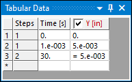
In this case the end time of the actual transient analysis is 30 seconds. Note that the Y displacement in the second step is deactivated.
In the Analysis Settings Details view, set the following for first step:
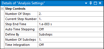
You can choose appropriate time step sizes for the second step (the actual transient). Make sure that time integration effects are turned on for the second step.
In the first step, inertia effects will not be included but velocity will be computed based on the displacement applied. In the second step, this displacement is released by deactivation and the time integration effects are turned on.
Initial Displacement ≠ 0, Initial Velocity ≠ 0: This is similar to case a. above except that the imposed displacements are the actual values instead of "small" values. For example if the initial displacement is 1 inch and the initial velocity is 2.5 inch/sec then you would apply a displacement of 1 inch over 0.4 seconds.
Specify two steps in your analysis. The first step will be used to establish initial displacement and velocity on one or more parts.
Choose a small end time (compared to the total span of the transient analysis) for the first step. The second step will cover the total time span.
Specify the initial displacement(s) on one or more faces of the part(s) as needed. This requires that you do not have any other boundary condition on the part that will interfere with rigid body motion of that part. Make sure that these displacements are ramped from a value of 0.
Deactivate or release the specified displacement load in the second step so that the part is free to move with the specified initial velocity.
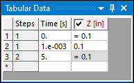
For example if you want to specify an initial Z velocity on a part of 0.5 inch/sec and have an initial displacement of 0.1 inch, then your first step end time = (0.1/0.5) = 0.2 second. Make sure that the displacement is ramped from a value of 0 at time = 0 so that you will get the required velocity.
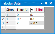
In this case the end time of the actual transient analysis is 5 seconds. Note that the Z displacement in the second step is deactivated.
In the Analysis Settings Details view, set the following for first step:
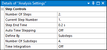
You can choose appropriate time step sizes for the second step (the actual transient). Make sure that time integration effects are turned on for the second step.
In the first step, inertia effects will not be included but velocity will be computed based on the displacement applied. In the second step, this displacement is released by deactivation and the time integration effects are turned on.
Initial Displacement ≠ 0, Initial Velocity = 0: This requires the use of two steps also. The main difference between b. above and this scenario is that the displacement load in the first step is not ramped from zero. Instead it is step applied as shown below with 2 or more substeps to ensure that the velocity is zero at the end of step 1.
Specify two steps in your analysis. The first step will be used to establish initial displacement on one or more parts.
Choose an end time for the first step that together with the initial displacement values will create the necessary initial velocity.
Specify the initial displacement(s) on one or more faces of the part(s) as needed. This requires that you do not have any other boundary condition on the part that will interfere with rigid body motion of that part. Make sure that this load is step applied, that is, apply the full value of displacements at time = 0 itself and maintain it throughout the first step.
Deactivate or release the specified displacement load in the second step so that the part is free to move with the initial displacement values.
For example if you want to specify an initial Z displacement of 0.1 inch and the end time for the first step is 0.001 seconds, then the load history displays as shown below. Note the step application of the displacement.
In this case the end time of the actual transient analysis is 5 seconds. Note that the Z displacement in the second step is deactivated.
In the Analysis Settings Details view, set the following for first step. Note that the number of substeps must be at least 2 to set the initial velocity to zero.
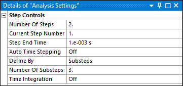
You can choose appropriate time step sizes for the second step (the actual transient). Make sure that time integration effects are turned on for the second step.
In the first step, inertia effects will not be included but velocity will be computed based on the displacement applied. But since the displacement value is held constant, the velocity will evaluate to zero after the first substep. In the second step, this displacement is released by deactivation and the time integration effects are turned on.
Apply Boundary Conditions
For this analysis type, loading is always step-applied (regardless of the setting of the Time Integration property). The Environment Context tab provides the various groups of loads, supports, and conditions.
In this analysis, the load’s magnitude can be constant or vary with time as defined in or as a . Details of how to apply a tabular or function load are described in Specifying Boundary Condition Magnitude. In addition, for more information about time stepping and ramped loads, see the Applying Stepped and Ramped Loads section.
Note:
You can use a Joint Load to kinematically drive a joint. See For the solver to converge, it is recommended that you ramp joint load angles and positions from zero to the real initial condition over one step.
Joint loads are not supported for the Samcef or ABAQUS solver.
Acceleration and/or Displacement can be defined as a base excitation only in a Transient Structural Analysis Using Linked Modal Analysis System.
Solve
When performing a nonlinear analysis, you may encounter convergence difficulties due to a number of reasons. Some examples may be initially open contact surfaces causing rigid body motion, large load increments causing non-convergence, material instabilities, or large deformations causing mesh distortion that result in element shape errors. To identify possible problem areas some tools are available under Solution Information object Details view.
Solution Output continuously updates any listing output from the solver and provides valuable information on the behavior of the structure during the analysis. Any convergence data output in this printout can be graphically displayed as explained in the Solution Information section.
You can display contour plots of Newton-Raphson Residuals in a nonlinear static analysis. Such a capability can be useful when you experience convergence difficulties in the middle of a step, where the model has a large number of contact surfaces and other nonlinearities. When the solution diverges, identifying regions of high Newton-Raphson residual forces can provide insight into possible problems.
Result Tracker is another useful tool that enables you to monitor displacement and energy results as the solution progresses. This is especially useful in the case of structures that may go through convergence difficulties due to buckling instability. Result Tracker is not available to the Samcef or ABAQUS solver.
Review Results
All structural result types except frequencies are available as a result of a transient structural analysis. You can use a Solution Information object to track, monitor, or diagnose problems that arise during a solution.
Once a solution is available you can contour the results or animate the results to review the response of the structure.
As a result of a nonlinear static analysis, you may have a solution at several time points. You can use probes to display the variation of a result item as the load increases.
Note: Fixed body-to-body joints between two rigid bodies will not produce a joint force or moment in a transient structural analysis.
Also of interest is the ability to plot one result quantity (for example, displacement at a vertex) against another result item (for example, applied load). You can use the Charts feature to develop such charts. Charts are also useful to compare results between two analyses of the same model. For example, you can compare the displacement response at a vertex from two transient structural analyses with different damping characteristics.