


Many important engineering flows involve swirl or rotation and Ansys Fluent is well-equipped to model such flows. Swirling flows are common in combustion, with swirl introduced in burners and combustors in order to increase residence time and stabilize the flow pattern. Rotating flows are also encountered in turbomachinery, mixing tanks, and a variety of other applications.
Information about rotating and swirling flows is provided in the following subsections:
For more information about the theoretical background of swirling and rotating flows, see Swirling and Rotating Flows in the Theory Guide.
When you begin the analysis of a rotating or swirling flow, it is essential that you classify your problem into one of the following five categories of flow:
axisymmetric flows with swirl or rotation
fully three-dimensional swirling or rotating flows
flows requiring a moving reference frame
flows requiring multiple moving reference frames or mixing planes
flows requiring sliding meshes
Modeling and solution procedures for the first two categories are presented in this section. The remaining three, which all involve “moving zones”, are discussed in Modeling Flows with Moving Reference Frames.
An overview of swirling and rotating flows is presented in the following sections:
Your problem may be axisymmetric with respect to geometry and flow conditions but still include swirl or rotation. In this case, you can model the flow in 2D (that is, solve the axisymmetric problem) and include the prediction of the circumferential (or swirl) velocity. It is important to note that while the assumption of axisymmetry implies that there are no circumferential gradients in the flow, there may still be nonzero swirl velocities.


When there are geometric changes and/or flow gradients in the circumferential direction, your swirling flow prediction requires a three-dimensional model. If you are planning a 3D Ansys Fluent model that includes swirl or rotation, you should be aware of the setup constraints listed in Coordinate System Restrictions. In addition, you might consider simplifications to the problem that might reduce it to an equivalent axisymmetric problem, especially for your initial modeling effort. Because of the complexity of swirling flows, an initial 2D study, in which you can quickly determine the effects of various modeling and design choices, can be very beneficial.
Important: For 3D problems involving swirl or rotation, there are no special inputs required during the problem setup and no special solution procedures. Note, however, that you may want to use the cylindrical coordinate system for defining velocity-inlet boundary condition inputs, as described in Defining the Velocity. Also, you may find the gradual increase of the rotational speed (set as a wall or inlet boundary condition) helpful during the solution process. This is described for axisymmetric swirling flows in Improving Solution Stability by Gradually Increasing the Rotational or Swirl Speed.
If your flow involves a rotating boundary that moves through the fluid (for example, an impeller blade or a grooved or notched surface), you must use a moving reference frame to model the problem. Such applications are described in detail in Introduction. If you have more than one rotating boundary (for example, several impellers in a row), you can use multiple reference frames (described in The Multiple Reference Frame Model) or mixing planes (described in Legacy Mixing Plane Model).
If you are modeling turbulent flow with a significant amount
of swirl (for example, cyclone flows, swirling jets), you should consider
using one of Ansys Fluent’s advanced turbulence models: the RNG  -
-  model, realizable
  -
-  model, or Reynolds
stress model. The appropriate choice depends on the strength of the
swirl, which can be gauged by the swirl number. The swirl number is
defined as the ratio of the axial flux of angular momentum to the
axial flux of axial momentum:
model, or Reynolds
stress model. The appropriate choice depends on the strength of the
swirl, which can be gauged by the swirl number. The swirl number is
defined as the ratio of the axial flux of angular momentum to the
axial flux of axial momentum:
 | (9–15) |
where  is the hydraulic radius.
For flows with weak to moderate swirl ( ), both the RNG
  -
-  model and the realizable
  -
-  model yield appreciable
improvements over the standard
model yield appreciable
improvements over the standard  -
-  model. See RNG k-ε Model and Realizable k-ε Model Swirl Modification for details about these models.
For highly swirling flows ( ), the Reynolds stress model (RSM)
is strongly recommended. The effects of strong turbulence anisotropy
can be modeled rigorously only by the second-moment closure adopted
in the RSM. See Reynolds Stress Model (RSM) Steps in Using a Turbulence Model for details about this model.
), the Reynolds stress model (RSM)
is strongly recommended. The effects of strong turbulence anisotropy
can be modeled rigorously only by the second-moment closure adopted
in the RSM. See Reynolds Stress Model (RSM) Steps in Using a Turbulence Model for details about this model.
For swirling flows encountered in devices such as cyclone separators and swirl combustors, near-wall turbulence modeling is quite often a secondary issue at most. The fidelity of the predictions in these cases is mainly determined by the accuracy of the turbulence model in the core region. However, in cases where walls actively participate in the generation of swirl (that is, where the secondary flows and vortical flows are generated by pressure gradients), non-equilibrium wall functions can often improve the predictions since they use a law of the wall for mean velocity sensitized to pressure gradients. See Near-Wall Treatments for Wall-Bounded Turbulent Flows in the Theory Guide for additional details about near-wall treatments for turbulence.
Recall that for an axisymmetric problem, the axis of rotation
must be the  axis and the mesh must lie on or above the
  line.
line.
In addition to the setup constraint described above, you should be aware of the need for sufficient resolution in your mesh when solving flows that include swirl or rotation. Typically, rotating boundary layers may be very thin, and your Ansys Fluent model will require a very fine mesh near a rotating wall. In addition, swirling flows will often involve steep gradients in the circumferential velocity (for example, near the centerline of a free-vortex type flow), and therefore require a fine mesh for accurate resolution.
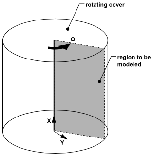
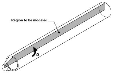
As discussed in Overview of Swirling and Rotating Flows, you can solve a 2D axisymmetric problem that includes the prediction of the circumferential or swirl velocity. The assumption of axisymmetry implies that there are no circumferential gradients in the flow, but that there may be nonzero circumferential velocities. Examples of axisymmetric flows involving swirl or rotation are depicted in Figure 9.10: Rotating Flow in a Cavity and Figure 9.11: Swirling Flow in a Gas Burner.
For axisymmetric problems, you must perform the following steps during the problem setup procedure. (Only those steps relevant specifically to the setup of axisymmetric swirl/rotation are listed here. You must set up the rest of the problem as usual.)
Enable the solution of the momentum equation in the circumferential direction by turning on the Axisymmetric Swirl option for Space in the General task page.
 Setup →
  General →
  Axisymmetric Swirl
Define the rotational or swirling component of velocity,
 , at
inlets or walls. Setup → Boundary Conditions
, at
inlets or walls. Setup → Boundary Conditions
Important: Remember to use the axis boundary type for the axis of rotation.
The procedures for input of rotational velocities at inlets and at walls are described in detail in Defining the Velocity and Velocity Conditions for Moving Walls.
The difficulties associated with solving swirling and rotating flows are a result of the high degree of coupling between the momentum equations, which is introduced when the influence of the rotational terms is large. A high level of rotation introduces a large radial pressure gradient that drives the flow in the axial and radial directions. This, in turn, determines the distribution of the swirl or rotation in the field. This coupling may lead to instabilities in the solution process, and you may require special solution techniques in order to obtain a converged solution. Solution techniques that may be beneficial in swirling or rotating flow calculations include the following:
(Pressure-based segregated solver only) Use the PRESTO! scheme (enabled in the Pressure list for Spatial Discretization in the Solution Methods Task Page), which is well-suited for the steep pressure gradients involved in swirling flows.
Ensure that the mesh is sufficiently refined to resolve large gradients in pressure and swirl velocity.
(Pressure-based solver only) Change the under-relaxation parameters on the velocities, perhaps to 0.3–0.5 for the radial and axial velocities and 0.8–1.0 for swirl.
(Pressure-based solver only) Use a sequential or step-by-step solution procedure, in which some equations are temporarily left inactive (see below).
If necessary, start the calculations using a low rotational speed or inlet swirl velocity, increasing the rotation or swirl gradually in order to reach the final desired operating condition (see below).
See Using the Solver for details on the procedures used to make these changes to the solution parameters. More details on the step-by-step procedure and on the gradual increase of the rotational speed are provided below.
Often, flows with a high degree of swirl or rotation will be easier to solve if you use the following step-by-step solution procedure, in which only selected equations are left active in each step. This approach allows you to establish the field of angular momentum, then leave it fixed while you update the velocity field, and then finally to couple the two fields by solving all equations simultaneously.
Important: Since the density-based solvers solve all the flow equations simultaneously, the following procedure applies only to the pressure-based solver.
In this procedure, you will use the button in the Solution Controls Task Page to turn individual transport equations on and off between calculations.
If your problem involves inflow/outflow, begin by solving the flow without rotation or swirl effects. That is, enable the Axisymmetric option instead of the Axisymmetric Swirl option in the General Task Page, and do not set any rotating boundary conditions. The resulting flow-field data can be used as a starting guess for the full problem.
Enable the Axisymmetric Swirl option and set all rotating/swirling boundary conditions.
Begin the prediction of the rotating/swirling flow by solving only the momentum equation describing the circumferential velocity. This is the Swirl Velocity listed in the Equations list in the Equations Dialog Box. Let the rotation “diffuse” throughout the flow field, based on your boundary condition inputs. In a turbulent flow simulation, you may also want to leave the turbulence equations active during this step. This step will establish the field of rotation throughout the domain.
Turn off the momentum equations describing the circumferential motion (Swirl Velocity). Leaving the velocity in the circumferential direction fixed, solve the momentum and continuity (pressure) equations (Flow in the Equations list in the Equations Dialog Box) in the other coordinate directions. This step will establish the axial and radial flows that are a result of the rotation in the field. Again, if your problem involves turbulent flow, you should leave the turbulence equations active during this calculation.
Turn on all of the equations simultaneously to obtain a fully coupled solution. Note the under-relaxation controls suggested above.
In addition to the steps above, you may want to simplify your calculation by solving isothermal flow before adding heat transfer or by solving laminar flow before adding a turbulence model. These two methods can be used for any of the solvers (that is, pressure-based or density-based).
Because the rotation or swirl defined by the boundary conditions can lead to large complex forces in the flow, your Ansys Fluent calculations will be less stable as the speed of rotation or degree of swirl increases. Hence, one of the most effective controls you can apply to the solution is to solve your rotating flow problem starting with a low rotational speed or swirl velocity and then slowly increase the magnitude up to the desired level. The procedure for accomplishing this is as follows:
Set up the problem using a low rotational speed or swirl velocity in your inputs for boundary conditions. The rotation or swirl in this first attempt might be selected as 10% of the actual operating conditions.
Solve the problem at these conditions, perhaps using the step-by-step solution strategy outlined above.
Save this initial solution data.
Modify your inputs (boundary conditions). Increase the speed of rotation, perhaps doubling it.
Restart the calculation using the solution data saved in step 3 as the initial solution for the new calculation. Save the new data.
Continue to increment the speed of rotation, following steps 4 and 5, until you reach the desired operating condition.