2.2. Modeling Rigid Bodies in a Multibody Analysis

Rigid bodies are widely used for numerical simulation of multibody dynamic applications. A rigid body can be connected to other rigid bodies via joint elements. It can also be connected to flexible bodies to model mixed rigid-flexible body dynamics.

In a finite-element model, certain relatively stiff parts can be represented by rigid bodies when stress distributions and wave propagation in such parts are not critical. An advantage of using rigid bodies rather than deformable finite elements is computational efficiency. Elements that belong to the rigid bodies have no associated internal forces or stiffness. The motion of the rigid body is determined by a maximum of six degrees of freedom (DOFs) at the pilot node.

For transient dynamic analyses, stiff bodies can excite high-frequency modes, resulting in a small time increment in order to obtain a stable solution. Rigid bodies do not, however, excite any frequency modes; therefore, using rigid bodies to represent stiff regions may allow a relatively large time increment.

The following topics about rigid body modeling are available:

2.2.1. Defining a Rigid Body

A rigid body in Mechanical APDL consists of a set of target nodes called rigid body nodes and a single pilot node. The associated target elements use the same real constant ID. The motion of the rigid body is governed by the degrees of freedom (DOFs) at the pilot node, allowing accurate representation of the geometry, mass, and rotary inertia of the rigid body.

2.2.1.1. Typical Rigid Body Scenarios

In most applications, rigid bodies start with discretized finite elements. The rigid body can be defined on the exterior of a pre-meshed body discretized by solid, shell, and beam elements (called underlying elements), as shown:

Figure 2.2: Rigid Body Definition With Underlying Elements

The 3D target element (TARGE170) and 2D target element (TARGE169) are applied on the exterior surface of the rigid body. To generate the target elements, issue ESURF.

The rigid body can also be a simple standalone body when the target elements do not overlap other elements (that is, have no underlying elements), as shown:

Figure 2.3: Rigid Body Definition Without Underlying Elements

You can generate target elements TARGE170 for a standalone 3D rigid body (AMESH) or target elements TARGE169 for a standalone 2D rigid body (LMESH).

The most efficient rigid body should contain a limited number of nodes which are either connected to other elements or subject to boundary conditions, as shown:

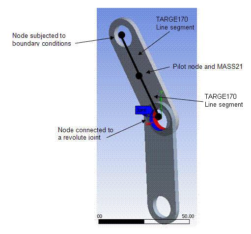
Figure 2.4: Rigid Body with a Limited Number of Nodes

The rigid body shown above contains three nodes which connect five elements (two 3D line segments, one pilot node segment, one MASS21, and one MPC184-Revolute).

Target element POINT segments (TSHAP,POINT) can be defined and used to apply boundary conditions (point loads, displacement constraints, etc.) on the rigid body surface where no predefined nodes exist.

2.2.1.2. Defining a Pre-meshed Body as a Rigid Body with RBGEN

Use the RBGEN command to define a pre-meshed body as a rigid body. The command generates target elements (TARGE169 for 2D or TARGE170 for 3D) on the exterior of a pre-meshed body discretized by solid, shell, and beam elements (called underlying elements), along with a pilot node . The target elements generated for the rigid body will have the same real constant ID as the pilot node target element. This ID should not be associated with any other rigid body.

Use the MESHOPT option to instruct RBGEN to delete the underlying elements or convert them to MESH200 elements.

Use the MASSOPT = 1 option to instruct RBGEN to to add a MASS21 element at the pilot node.

The required arguments for RBGEN commands:

Pilot node number (P0)
Element component need to defined as rigid body (ELSET)
Nodal component to defined as pin-type/tie-type (NDSET)
Target element type (ITTY)
Real constant ID (RID)
Mesh option (MESHOPT)
Mass option (MASSOPT)

These inputs are discussed in detail below.

Pilot node (P0)

Each rigid body is associated with a pilot node, You may specify the pilot node, or request automatic generation of the pilot node at the centroid location of a given element component.

Element component (ELSET)

Use argument ELSET to specify the component composed of the elements to be defined as rigid body. The rigid body can be defined on the exterior of a pre-meshed body discretized by solid, shell, and beam elements.

Node component (NDSET)

Use arguments NDSET to specify the component composed of the nodes to be added to a rigid body as Target element POINT segments (TSHAP,POINT)and to be defined as Pin-type/Tie-type node .

Target Element Types (ITTY)

By default, the program automatically creates the next available target element types required for the rigid body. However, you may use the ITTY arguments to specify the target element types. If you specify the element types using ITTY, you must also set KEYOPT(2) = 1.

Real ID (RID)

By default, the program automatically defines the next available real constant ID number. However, you may specify a user-defined real ID to the rigid target elements using the RID option.

Mesh Option (MESHOPT)

By default, the value of MESHOPT is set to 0 and the program automatically deletes the underlying elements.

However, you may set MESHOPT to 1 to convert the underlying elements to MESH200 and keep it for further application of load.

Mass Option (MASSOPT)

By default, the MASSOPT value is set to 0 and the program does not generate the MASS21 elements. As in static analysis the rigid bodies do not contribute mass to the finite element system.

However, you may set the MASSOPT value to 1 to generate a MASS21 element at the pilot node. By default, this element is located at the center of mass, however you may define the pilot node location. Mass and rotary inertias are defined automatically through the real constant of MASS21. In dynamic analysis, the mass and rotary inertia of the rigid body play important roles in the dynamic response. For more details refer to Defining Rigid Body Mass and Rotary Inertia Properties.

The following example input shows typical commands used to define a body meshed with SOLID186 as the rigid target body.

Figure 2.5: Type 1 and 2 are base elements meshed with SOLID186

Esel,s,type,,2
cm,erigid,elem
allsel,all
RBGEN,10000,erigid,,,2

Figure 2.6: Type 6 are Rigid Target Elements and the Starred Node (*) is the Pilot Node

Additional Guidelines for RBGEN

Keep the following points in mind when creating a rigid body using RBGEN.

Do not associate the pilot node and nodes meshed with TSHAP,POINT defined as pin-type or tie-type to any other rigid bodies.
Use ALLSEL,ALL before RBGEN.

2.2.1.3. Target Element Key Option Setting for Defining a Rigid Body

Each rigid body contains target elements defined by the same real constant ID. The target elements can be defined via different element type IDs, however, you must set KEYOPT(2) = 1 on all of the target elements. This KEYOPT setting causes Mechanical APDL to build internal multipoint constraints (MPC) to enforce kinematics of the entire rigid body.

You can also combine different target segment types for each rigid body. However, you cannot mix 2D with 3D target elements.

2.2.1.4. Defining a Rigid Body Pilot Node

In addition to the rigid body nodes, each rigid body also must be associated with a rigid body pilot node. The target element defining the pilot node must use the same real constant ID as the other target elements which constitute the rigid body. The real constant ID identifies each rigid body, and Mechanical APDL builds internal multipoint constraints (surface-based rigid constraints) during solution.

The pilot node, unlike the other segment types, is used to define the degrees of freedom for the entire rigid body. This node can be any of the target element nodes, but it does not have to be. All possible rigid motions of the rigid body will be a combination of a translation and a rotation around the pilot node. The pilot node provides a convenient and powerful way to assign boundary conditions such as rotations, translations, moments, temperature, voltage, and magnetic potential on the entire rigid body. The pilot node can be connected to point mass, follower, and deformable elements. For a transient analysis, you can simply locate the pilot node at the gravity center of the rigid body if the center of mass is known.

2.2.1.5. Defining Rigid Body Mass and Rotary Inertia Properties

For multibody dynamics, the mass and rotary inertia of the rigid body play important roles in the dynamic response. In Mechanical APDL, the target elements which define rigid bodies do not contribute mass to the finite element system. The most effective way to contribute mass is to add the point mass element MASS21 on the gravity center of the rigid body when the center of mass and rotary inertia properties of the actual rigid body can be estimated. You can specify the rigid body mass and rotary inertia for MASS21. The node of the MASS21 element is usually connected to the pilot node, although it can be connected to any one of the rigid body nodes. The point mass node is often defined in a local coordinate system which is parallel to the rotary principal axes.

Sometimes, the location of gravity center, the mass, and rotary inertia cannot be easily estimated. In such cases, you can use the premeshed body to account for mass distribution for the rigid body (as shown in Figure 2.2: Rigid Body Definition With Underlying Elements). The discretized elements can be pure elastic solid, shell, or beam elements.

For each rigid body, you can perform the following steps:

Select the associated elements (ESEL)
Specify the option for precalculating masses (IRLF,-1).
Perform a partial element solution and calculate inertia relief terms (PSOLVE,ELFORM).
Get the mass properties (*GET), as follows:

GET, `Par`*, ELEM, 0, Item1, IT1NUM, Item2, IT2NUM
Item1	IT1NUM	Description	Symbol
MTOT	X, Y, Z	Total mass components.	M_x, M_y, M_z
MC	X, Y, Z	Mass centroid components.	X_c, Y_c, Z_c
IPRIN	X, Y, Z	Principal centroidal moments of inertia.	I_xx, I_yy, I_zz
IANG	XY, YZ, ZX	Angles of the principal axes.	θ_xy, θ_yz, θ_xz

Based on the precalculated mass properties, you can easily define the point mass element. The node is defined in the local coordinate system, as shown:

X_c, Y_c, Z_c, θ_xy, θ_yz, θ_xz

The mass properties are specified by real constants:

M_x, M_y, M_z, I_xx, I_yy, I_zz

Set MASS21 KEYOPT(2) = 1 so that the point mass element coordinate system is initially parallel to the nodal coordinate system and rotates with the nodal coordinate rotations during a large-deflection analysis.

2.2.2. Rigid Body Degrees of Freedom

The pilot node has both translational and rotational degrees of freedom (DOFs). The active DOFs at the pilot node depend on the defined type of target elements. Use TARGE169 for a 2D rigid body which contains UX, UY and ROTZ DOFs. Use TARGE170 for 3D rigid body which contains UX, UY, UZ and ROTX, ROTY, ROTZ DOFs.

The DOFs of rigid body nodes are based on the DOFs of the connected elements and applied boundary conditions (BCs). Rigid body nodes that connect to solid elements involve only the translational degrees of freedom. Rigid body nodes that connect to shell, beam, follower, and joint elements also involve the rotational DOFs.

For standalone rigid body nodes not connected to any other elements, the associated DOFs are subject to applied boundary conditions, as shown:

Figure 2.7: 2D Rigid Body DOFs Subject to Applied Boundary Conditions

The node has DOF UX if a constraint or a force is applied in the X direction. If there are no applied BCs, the standalone rigid body nodes have no DOFs; in such a case, Mechanical APDL simply updates the position of the nodes based on the kinematics of the rigid body.

The DOFs for a rigid body can also be controlled via KEYOPT(4) of the target element (TARGE169 or TARGE170). The key option offers additional flexibility by fully or partially constraining the DOFs for the rigid body.

Examples

In the following figure, a rigid sphere is defined by 8-node quadrilateral segments and a pilot node. Two beam elements are connected to the rigid surface in the XY plane, as shown by the dotted lines. The pilot node is located at the global Cartesian origin and is subjected to rotation ROTZ.

For the DOFs of the rigid body, selecting three rotational DOFs along with three translational DOFs rotates the beams, as shown. Because the beams are fully connected to the rigid sphere, they rotate with the sphere.

Figure 2.8: Rigid Sphere Translational DOFs + Rotational DOFs

Selecting only the three translational DOFs for the rigid body, as shown in the following figure, does not rotate the beams because they are connected only in their translational DOFs; therefore, the connection acts as a hinge.

Figure 2.9: Rigid Body Translational DOFs Only

Determining the DOFs for each rigid body node is important because the internal multipoint constraints are built solely on the resulting DOFs.

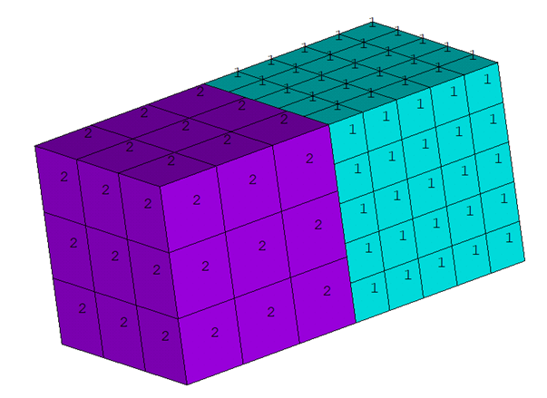
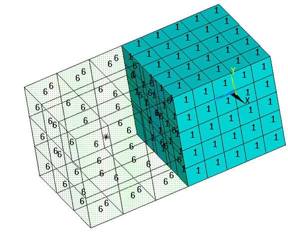
Pin-type and tie-type nodes are also useful tools for defining a solid-like rigid body, that is, where nodes do not possess rotational degrees of freedom. Below is an example comparing pin-type nodes and tied-type nodes when a single block is rotated by 45 degrees with respect to its center.

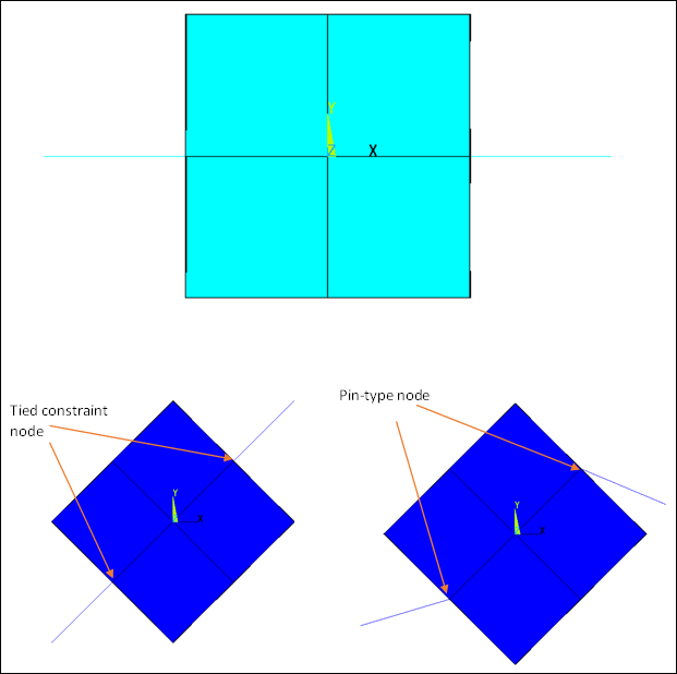
Figure 2.10: Pin-type and Tie-type Nodes

Tie node is defined by setting target KEYOP(7) = 0 on the target element.

Pin node is defined by setting point segment type and target KEYOPT(7) = 1.

Pin node or tie node definition will override target KEYOPT(4) on its own. It can coexist with other types of constraints within the same rigid pair. This implies that nodes which are defined by TSHAP,POINT and KEYOPT(7) = 0 or 1 for tie or pin type node. In addition, the degrees of freedom of other nodes are controlled by KEYOPT(4) within the same rigid pair. Pin-type nodes may not be shared with another rigid body.

2.2.3. Rigid Body Boundary Conditions

Constrained boundary conditions (BCs) for the rigid body are usually applied on the rigid body pilot node. Reaction forces can be obtained for DOFs at the constrained nodes. A combination of rigid body constraints and constrained boundary conditions applied to several rigid body nodes other than the pilot node can lead to overconstrained models. In such cases, Mechanical APDL issues overconstraint warnings and attempts to remove the redundant constraints if possible. If the specified BCs are not consistent with the rigid body constraint, the model becomes inconsistently overconstrained. You must verify the overconstrained model and prevent conflicting overconstraints.

2.2.3.1. Defining Rigid Body Loads

You can apply point loads on any rigid body nodes and pilot node. Follower force (FOLLW201) can be defined at those nodes, and the direction of forces is determined by the rotation of the nodes.

You can apply surface loads on surface effect elements SURF153 and SURF154 which fully or partially override loads on the surface of the rigid body.

Loads on a rigid body are assembled from contributions of all loads on nodes and elements connected to the rigid body.

2.2.4. Representing Parts of a Complex Model with Rigid Bodies

Using rigid bodies to represent certain portions of a complex model is more efficient than using flexible finite elements. In the early stage of finite element model development, you can treat certain stiff parts or discretized elements that are far away from the region of interest as the rigid bodies. In a later stage, you can remove the rigid body definition and add the flexible discretized elements back for a detailed and accurate finite element analysis.

By selecting or deselecting target elements or the flexible finite elements, you can easily switch back and forth between rigid body and flexible body definition.

The following table shows the general steps involved when defining a rigid body as compared to defining a flexible body:

Table 2.1: Rigid Body vs. Flexible Body Definition

Rigid Body Definition Process	Flexible Body Definition Process
Select the associated finite elements with defined mass density. Perform a partial element solution to obtain mass properties. Add a point mass element to the center of rigid body. Add a target element whose node (pilot node) shares the point mass node. Generate target elements on the exterior surface of the pre-mesh body. Unselect the associated finite elements. Connect joint elements to target nodes.	Unselect the relevant point mass and target elements. Reselect the associated finite elements. Define the material properties for the flexible body. Define a pilot node at one end of the joint. The pilot node connects the joint to the rest of the body. Select the nodes on the exterior surface of the body that you want to connect to this pilot node. Create target elements on this surface. For each body-joint connection, repeat steps 4 through 6. For more information, see Connecting Bodies to Joints.

Rigid Body Definition Process

Flexible Body Definition Process

Select the associated finite elements with defined mass density.
Perform a partial element solution to obtain mass properties.
Add a point mass element to the center of rigid body.
Add a target element whose node (pilot node) shares the point mass node.
Generate target elements on the exterior surface of the pre-mesh body.
Unselect the associated finite elements.
Connect joint elements to target nodes.

Unselect the relevant point mass and target elements.
Reselect the associated finite elements.
Define the material properties for the flexible body.
Define a pilot node at one end of the joint. The pilot node connects the joint to the rest of the body.
Select the nodes on the exterior surface of the body that you want to connect to this pilot node.
Create target elements on this surface.

For each body-joint connection, repeat steps 4 through 6. For more information, see Connecting Bodies to Joints.

2.2.5. Connecting Joint Elements to Rigid Bodies

Joint elements can be connected to any rigid body nodes and the pilot node. You can define connections between rigid bodies, or between a rigid body and a flexible body.

Caution: Redundant constraints are most likely to occur when two rigid bodies are connected to more than one joint element.

2.2.6. Modeling Contact with Rigid Bodies

Contact between two rigid bodies is modeled by specifying a contact surface on one rigid body and a target surface on another rigid body. Use either the augmented Lagrange algorithm or penalty algorithm (KEYOPT(2) on the contact element) for modeling contact between rigid bodies to avoid redundant overconstraint between rigid body constraints and contact constraints.

You cannot use the multipoint constraint (MPC) algorithm (KEYOPT(2)) and bonded or no-separation contact behavior (KEYOPT(12)) to connect two rigid surfaces; doing so would cause the model to be overconstrained, resulting in an abnormal termination of the analysis. You can simply replace the bonded contact pair by adding an additional rigid body which connects two pilot nodes.

Mechanical APDL allows two rigid bodies that are connected or overlap each other through rigid body nodes or the pilot node. To prevent overconstraints, the program merges two rigid bodies into one rigid body internally and treats the second pilot node as a regular rigid body node.

MPC bonded contact between a flexible body and a rigid body is possible. The contact surface in an MPC bonded contact pair, however, should always belong to the flexible body; otherwise, the MPC bonded constraints and rigid body constraints are redundant.