The trend in modern CFD goes towards large-scale, unsteady simulations. For Scale Resolving Simulations (SRS, for example, LES) in industrial applications, meshes with billions of cells are required, and simulations are run on thousands of CPUs. To facilitate such simulations, massive parallel mesh generation is needed as well, where meshing must be robust with limited user interaction. Furthermore, SRS requires isotropic cells in order to resolve transported eddies, both in the bulk and also close to the wall.
The Rapid Octree mesher is based on massively parallel algorithms and data structures. It allows you to use an existing boundary geometry to generate a new volume mesh that is based on cube cells, such that the resulting meshes are mostly isotropic. At boundaries, the geometry is approximated by snapping or projecting vertices onto the surface if possible, but defeatured if under-resolved by the prescribed mesh size. Rather than capturing every single geometric feature, the paradigm is to maintain robust cell quality to enable stable simulations.
A typical target application for the Rapid Octree mesher is external aerodynamics for which a faceted geometry of the object and the dimensions of the outer bounding box (for example, a wind tunnel) are provided. Meshes for internal flows can be easily generated as well.
The following sections are described in this chapter:
To begin, you must read in a boundary geometry that provides a triangulated surface; this can be an enclosed surface mesh or a volume mesh. (Note that this original mesh data will be cleared during this process.) Then you can access the Rapid Octree meshing algorithm through the Mesh menu:
Mesh → Rapid Octree...
This opens the Rapid Octree dialog box.
To generate the octree mesh, you must define settings in the three top-level group
boxes (which are described in the following sections), and click the
button at the bottom of the Rapid
Octree dialog box. If the resulting mesh is not satisfactory, you can read the
mesh again or (if the mesh was generated from a geometry object or mesh object) you can
restore the object state (including its surfaces) as it was prior to the meshing operation
by entering the following text command:
/mesh/rapid-octree/undo-last-meshing-operation; then you can
regenerate the mesh with revised settings.
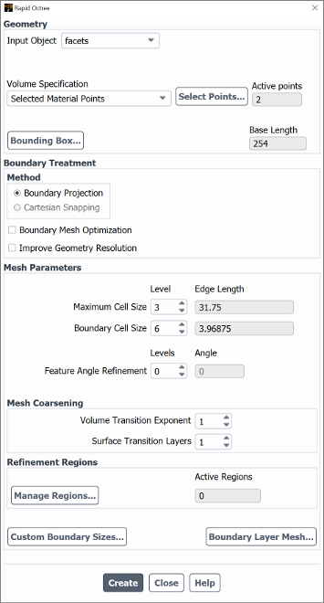
The Geometry group box allows you to specify the input object, specify the volume to be meshed, define the bounding box for the geometry, and display the base length (which is the main size for all subsequent mesh size specifications).
See the following for details:
You can make a selection from the Input Object drop-down list to specify that the geometry is a particular geometry object or a mesh object; alternatively, you can select none so that all available surface zones are used. Note that when a geometric object is selected and meshed, a corresponding mesh object is created.
You must indicate the region to be meshed by making a selection from the Volume Specification drop-down list. These selections will result in the creation of a single volume / cell zone, unless otherwise noted.
Note: If you selected a mesh object for the Input Object and want to use volumetric regions as part of the Volume Specification, you must compute the volumetric regions, as described in Volumetric Region Management.
The following selections are available from the Volume Specification drop-down list:
Select Bound by Geometry for internal flows, so that the volume inside the geometry is meshed.
Select Bound by Bounding Box for external flows, so that the volume between the bounding box and the geometry is meshed. Note that the face zones that are created for the sides of this bounding box are named tunnel-<dom_ext>, where <dom_ext> represents the domain extent (tunnel-xmax, tunnel-xmin, tunnel-ymax, and so on).
Select Filled from Point if you want to define the coordinates of a point (in the X, Y, and Z fields) located in the region to be meshed. The point can be either within the geometry for internal flows, or between the bounding box and the geometry for external flows.
Select Selected Material Points if you want to generate disconnected cell zones (based on the existing volumetric regions) by defining and selecting material points within the various regions. To connect the resulting cell zones, you will need to create non-conformal mesh interfaces in the solution mode (as described in Using a Non-Conformal Mesh in Ansys Fluent). Note that the Selected Material Points selection does not require a watertight geometry. It is available regardless of what you selected from the Input Object drop-down list:
If you selected a geometry object or a mesh object for the Input Object, a mesh object will be created for each zone, since the zones will not be conformally connected.
If you selected none for the Input Object, separate mesh objects will not be created for each zone; instead, all generated cell and face zones will be stored as unreferenced. All other entities (objects, edges, cell zones, and so on) in the session will be deleted in the process.
If the regions are separated by face zones of type interface, each face zone will be split into two zones that have -nci:<ID> appended to the original name.
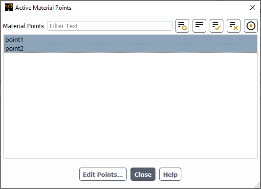
To complete the setup for the Selected Material Points selection, you must click the button and select material points in the Active Material Points dialog box that opens. These material points should be located in the separate regions you want to mesh. If you have not already created any material points, you can do so by clicking the button in the Active Material Points dialog box, and then using the Material Points dialog box that opens (as described in Creating Material Points). As you select material points, the total number is updated in the Active points field in the Rapid Octree dialog box.
Tip:It is recommended that you use one level of angular refinement for interfaces with corners, to promote better matching between the resulting cell zones.
If the geometry is not watertight, there can be cases in which the defined material points are not separated completely by the geometry. This can result in the creation of fewer cell zones than you intended. You can consider closing the geometry by creating patches (for example, using SpaceClaim). Such patches do not need to be stitched to the rest of the geometry.
You may want to enable the Improve Geometry Resolution option along with the Selected Material Points selection, as it can improve the interface matching between the cell zones. For further details, see Improve Geometry Resolution.
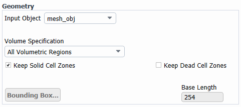
If you have selected a mesh object from the Input Object drop-down list, you can select the name of a particular volumetric region. The X, Y, and Z coordinates provide information about the location of the point that is used to generate the mesh.
Select All Volumetric Regions if you want to generate disconnected cell zones based on all of the existing volumetric regions. Note that this selection should only be used if you have a watertight geometry. It is available if you have selected a mesh object from the Input Object drop-down list. A mesh object will be created for each cell zone, since the zones will not be conformally connected. If mesh objects are separated by face zones of type interface, each face zone will be split into two zones that have -nci:<ID> appended to the original name; these zones can be used to create a non-conformal mesh interface in the solution mode (as described in Using a Non-Conformal Mesh in Ansys Fluent).
With this selection, you can enable options in order to Keep Solid Cell Zones and/or Keep Dead Cell Zones in the resulting mesh.
Tip: It is recommended that you use one level of angular refinement for interfaces with corners, to promote better matching between the zones.
Tip: Regardless of what you select from the Volume Specification drop-down list, if the meshing fails, you can try to change the settings so that the coordinates of the point used to generate the mesh is further away from any given boundary than the cell size defined for that boundary. If you can redefine the coordinates of the point, you can increase the distance from the boundaries; otherwise, you can decrease the cell size on the nearest boundaries. If the latter change is still unsuccessful or undesirable, you can instead use the Selected Material Points method described previously.
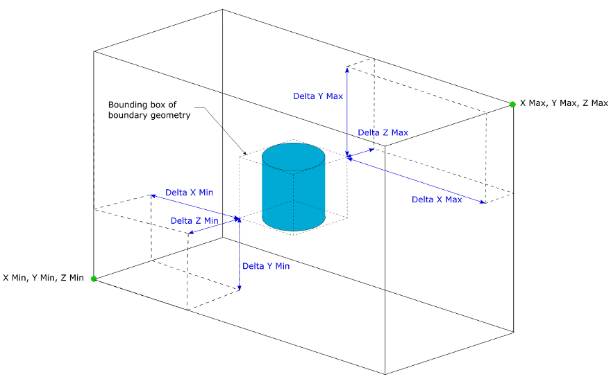
A bounding box is used to define the Rapid Octree meshing region. You can define the box by specifying the absolute extents (min / max x, min / max y, min / max z), or by specifying the offset relative to a box around one or more face zones (delta min / max x, delta min / max y, delta min / max z). The input geometry you want to mesh must be within this bounding box. For external flows, you will size the box to represent the extents of your flow domain (for example, the dimensions of the wind tunnel), with your geometry located appropriately; for internal flows, you will ensure that the box merely encompasses the geometry.
Note: The bounding box is not available when you select All Volumetric Regions or a particular volumetric region from the Volume Specification drop-down list, as the meshing region is automatically defined and does not require your input.
In the Rapid Octree dialog box, click the button to open the Bounding Box dialog box.
Perform the following steps:
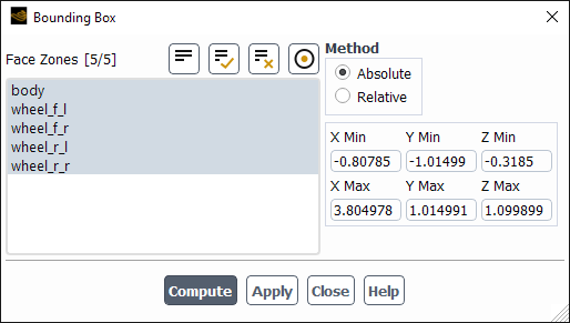
Select the Face Zones you want within the bounding box.
Select the Method by which you will define the box:
Absolute: after selecting this method, click to calculate the extents of a bounding box based on the selected face zones and display the relevant coordinates as a minimum (X Min, Y Min, Z Min) and maximum (X Max, Y Max, Z Max). You can then adjust these values to make the box larger or smaller.
Relative: after selecting this method, adjust the minimum offset (Delta X Min, Delta Y Min, Delta Z Min) and the maximum offset (Delta X Max, Delta Y Max, Delta Z Max) from the selected face zones.
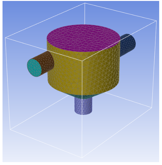
Click to create the bounding box and display it with the selected face zones in the graphics window.
Click to return to the Rapid Octree dialog box.
The Base Length is a non-editable field that reports the maximum extent of the bounding box and serves as the base length scale in the mesh generation process. All subsequent size specifications are based on it. The level specifications correspond to a division of the base size by the power of two to the given level.
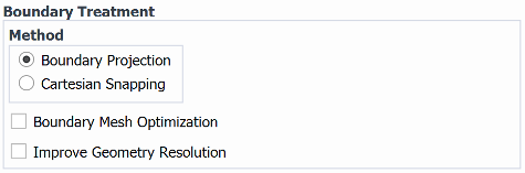
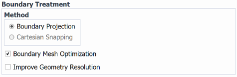
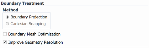
In the Boundary Treatment group box, the Method list allows you to choose between the Boundary Projection and Cartesian Snapping methods. Cartesian Snapping can only handle a constant size boundary mesh, so there are no other related controls in the dialog box; it is not available if you have selected All Volumetric Regions from the Volume Specification drop-down list. For Boundary Projection, it is possible to refine the surface mesh according to feature angles and/or local size by using the button, as described in Mesh Parameters.
Neither approach will capture feature lines in the model. This defeaturing will always be in the length scale of the boundary mesh size. The Cartesian Snapping approach is slightly faster than the Boundary Projection approach, but is not as good at representing thin structures.
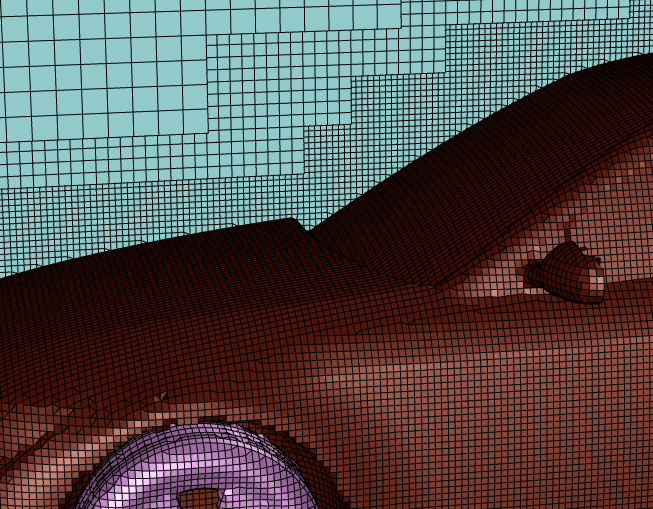
When using the Boundary Projection treatment method, you can enable the Boundary Mesh Optimization option in order to specify that the cells in the layer adjacent to boundary zones are optimized in terms of orthogonal quality at the time of meshing. When applied along with multiple prismatic layers (see Boundary Layer Mesh), note that the optimization is performed on the cells prior to their being split into the prismatic layers.
Important: This boundary mesh optimization is a very expensive process and will increase the mesh generation time significantly. It is not generally recommended, but may be necessary in some cases (for example, complex cases with multiple prismatic layers).
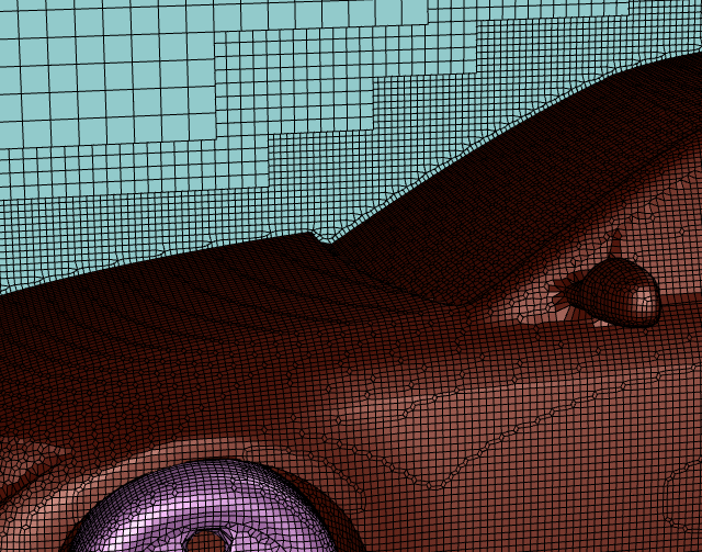
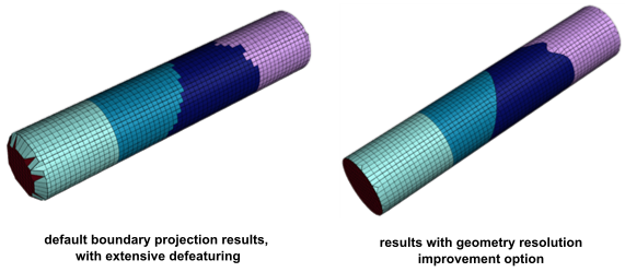
A known limitation of the Rapid Octree mesher is that defeaturing can occur at inlets, outlets, interior boundaries, and so on, such that the surface area of a generated boundary does not exactly match that of the original geometry. You can attempt to minimize such defeaturing by assigning boundary types, refining the mesh, and/or defining boundary conditions (as described in Limitations of the Rapid Octree Mesher). If such attempts are not sufficient, as part of the Boundary Projection treatment method you can enable the Improve Geometry Resolution option. This option applies an iterative projection of boundary faces onto the geometry, with the goal of minimizing the distance of the boundary face centroid to the geometry. This “face projection” is then internally iterated with mesh smoothing steps to improve the cell quality.
Note: The Improve Geometry Resolution option is an expensive process and will increase the mesh generation time significantly (for example, by a factor of 4).
Note:
Although the capturing of corners and face zone boundaries is improved significantly by using the Improve Geometry Resolution option, there can still be defeaturing. This can especially affect the capturing of face zone boundaries, most noticeably when the adjacent cells have nonuniform sizes. It is recommended that you check the mesh for such defeaturing, in order to avoid errors due to inaccurate boundary conditions.
For complex geometries, the Improve Geometry Resolution option can lead to significant deterioration of cell quality. It is therefore augmented with an automatic mesh repair step at the end of the mesh generation. Since this step can significantly increase the mesh generation time when there are large numbers of bad cells, it is only executed if the number of bad cells is below a threshold of 500. If this threshold is exceeded, you will receive a warning in the console, and you can try to address the issue by performing the following:
You can manually initiate a mesh repair. It is recommended that you first change the quality method to
inverse-ortho-qualitythrough thereport/quality-methodtext command; then you can perform the mesh repair on selected cells zones by using themesh/modify/auto-node-movetext command. For further details, seemesh/in the Fluent Text Command List.You can delete the bad cells by using the following text command for specified cell zones:
mesh/rapid-octree/delete-poor-quality-cells. When a cell is deleted, new face zones of type symmetry are created for the adjacent cells on the faces that were shared with the deleted cell. This text command should be used with care in order to avoid unwanted effects during the solution (such as solution errors due to bad geometry representation, or even solver divergence).
The Mesh Parameters group box allows you to define global mesh sizes by adjusting the Level for the following: the Maximum Cell Size specifies a maximum size for the mesh; and the Boundary Cell Size specifies the sizing on the geometry. Based on the values you enter, the Edge Length values will be updated for your review. Note that due to the nature of the octree method, only certain cell size values can be represented by the mesh; the available sizes are obtained by dividing the base size by the power of two to the given number of levels.
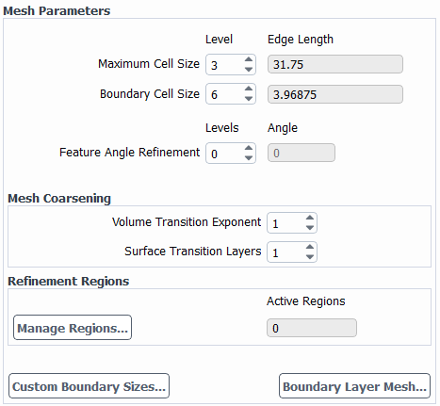
When using the Boundary Projection treatment method, you can define the Feature Angle Refinement fields as a global setting, so that the surface cell size is refined automatically wherever faces meet at an angle that is equal to or less than the specified Angle. At those locations, the boundary mesh is refined according to the given number of refinement Levels. Note that the Levels value is not absolute (like the Boundary Cell Size value), but is relative to the Max Size in the Surface Sizing dialog box. The Surface Sizing dialog box also allows you to set a unique local Angular Refinement for individual or groups of zones. For further details, see Custom Boundary Sizes).
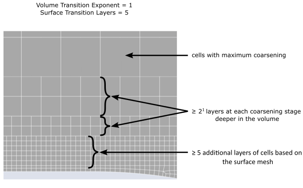
The Mesh Coarsening group box provides fields that control how the mesh coarsens as it proceeds from the geometry to deeper within the fluid volume. You can adjust the Volume Transition Exponent to control the transition from the fine cells near the surfaces to the coarse cells in the volume: enter 0 for the fastest possible transition, or higher numbers for a slower transition; as the value increases, so too will the thickness of cell layers of the same size at each stage of the transition. The number of layers at each intermediate stage of coarsening will be at least 2 to the power of the number you enter here. You can also set the Surface Transition Layers to define the minimum number of layers of constant-size cells that are added to the layer adjacent to the surfaces of the geometry; these cells are generally isotropic, with the dimensions determined by the surface mesh.
Finally, you can use the buttons at the bottom of the Mesh Parameters group box to set the following:
To refine specific regions of the mesh, click the button in the Refinement Regions group box to open the Rapid Octree Refinement Regions dialog box. There you can define the refinement regions and manage them.
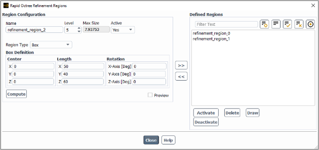
To begin creating a region, you can provide a Name for the definition. Then adjust the Level, to produce your desired Max Size for the cells in this region.
Next, select the Region Type and define it's extents and orientation. You can choose from the following:
Box
For a box, you define the Center coordinates and the Length in each of the coordinate axes. You can also define Rotation values about each of the coordinate axes, using the right-hand rule; note that the X-Axis rotation is applied first, then the Y-Axis rotation, and finally the Z-Axis rotation.
Frustum
This shape is a frustum of a cone, that is, a tapered cylinder. You define the coordinates of the centers of the circular faces at the ends (Center 0 and Center 1), as well as the Radii of the frustum at these points (Radius 0 and Radius 1, respectively).
To get good initial values for your box or frustum definition, you can click on a face zone (or multiple face zones, if you hold the Ctrl key) in the graphics display, and then click the button so that the region is sized to encompass the selected zone(s).
Enable the Preview option to automatically display your region in the graphics display. The shape will be translucent and gray, with a red cube in the center that represents the Max Size of the cells.
Tip: Note that when clicking on face zones and/or previewing the refinement region, you may need to adjust what face zones are displayed by using the Display Grid dialog box (as described in Generating the Mesh Display Using the Display Grid Dialog Box).
Click the button to save your settings. The name will be listed under Defined Regions, as well as whether it is inactive (in brackets).
You can repeat the previous steps to create additional definitions for refinement. At any point you can make a single selection from the Defined Regions list to display the settings in the fields of the Region Configuration group box. After reviewing the settings, you can: choose to allow it to remain as is; edit the settings as necessary and click the button to save it again; or click the button or the button to delete it. You can also make selections from the Defined Regions list and use the or buttons to determine whether they are active, and/or them in the graphics display. Note that the Active Regions field in the Rapid Octree dialog box displays the number of active refinement regions defined in the Defined Regions list.
When using the Boundary Projection treatment method, you can click the button to open the Surface Sizing dialog box, and there define size functions for the geometry, as well as local Angular Refinement settings.
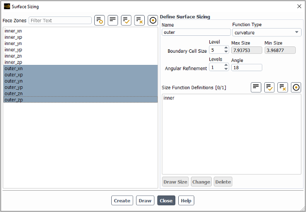
You can use the Surface Sizing dialog box to do the following:
To create a function, make selections in the Face Zones list or by clicking the mouse button on zones in the graphics window. After selection, enter a Name for the sizing function, and define a refinement Level for the Boundary Cell Size. The default selection of soft for the Function Type specifies that the global Feature Angle Refinement settings in the Rapid Octree dialog box are overwritten, so that no refinement is applied based on the angles at which faces meet; as an alternative, you have the option of selecting curvature for the Function Type and then defining local Angular Refinement settings for individual or groups of zones, so that additional Levels of refinement are applied relative to the Max Size. By clicking Create, the function is defined and added to the Size Functions list.
Each size function can include multiple face zones. The default level (for selected or unselected face zones) is the value specified for the Boundary Cell Size in the Rapid Octree dialog box. A size function can thereby also specify a coarser grid than the default, but not coarser than the Maximum Cell Size.
If a face zone is assigned to more than one size function, a warning is issued during mesh creation and the minimum specified level is used.
After a size function is created, it can be selected from the Size Functions list to display the settings, such as the Max Size. You can then perform the following:
Click the button to display small cubes on the face zones of the size function in the graphics window. These cubes indicate the size of the mesh. If a feature angle refinement is also specified, smaller cubes indicate the minimum cell size on that boundary zone.
Adjust the settings (zones, name, level and/or feature angle refinement) and click to revise the size function.
Click to delete the selected size function.
When using the Boundary Projection treatment method, by default a single layer of prismatic cells is generated at boundary zones, and these cells are generally isotropic. You have the option of defining multiple prismatic layers for specific boundary zones, so that this original isotropic layer is instead divided into many anisotropic layers at the time of meshing. This allows you to increase the mesh resolution perpendicular to the anticipated streamwise direction without overly increasing the cell count. It is an alternative to creating such layers after meshing by using other tools in the meshing mode or by using mesh adaption in the solution mode; it also allows you to combine this splitting with boundary mesh optimization (see Boundary Mesh Optimization), which can be helpful for complex cases.
When using this feature, you will define the total number of anisotropic prism layers that you want for a given boundary zone or group of boundary zones, along with other settings that determine the heights of the various layers.
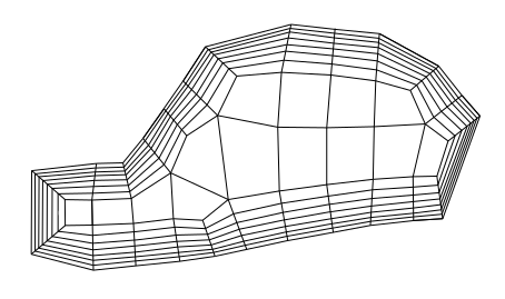
Important: It can be helpful to keep in the mind that with the Rapid Octree mesher, the anisotropic prism layers are not created at the boundaries as a first step before the remainder of the interior is meshed (as is common with other meshing methods), but instead a preliminary interior mesh is created first and then the cell layers near the boundaries are divided and/or adjusted to produce the anisotropic layers.
To define multiple prismatic layers at the boundaries, perform the following steps:
Select Boundary Projection from the Method list in the Boundary Treatment group box.
(Optional) You can enable the Boundary Mesh Optimization option for complex cases. For further details, see Boundary Mesh Optimization.
Define the other settings in the Rapid Octree dialog box, such as the Boundary Cell Size and Feature Angle Refinement, so that you get appropriate values when you initialize the prism layer settings (as described in a later step).
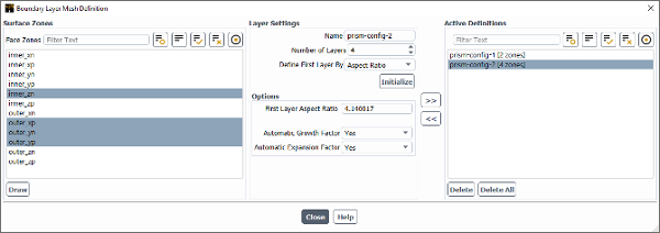
Click the button to open the Boundary Layer Mesh Definition dialog box.
Here you can repeatedly perform the following steps to define the prism layer settings for individual or groups of boundary zones:
Select one or more Face Zones.
(Optional) Click the button in the Surface Zones group box to display the selected zones in the graphics window, so that you can confirm they are the intended zones.
In the Layer Settings group box, enter a Name for this layer settings definition.
Enter the total Number of Layers that you want produced from the original isotropic layer adjacent to the selected Face Zones.
Make a selection from the Define First Layer By list to specify how you want to define the first anisotropic layer:
Select Height if you know the absolute height you would like for the first prism layer.
Select Aspect Ratio if you know the aspect ratio (that is, the base length of the cell divided by the height) you would like for cells in the first prism layer.
Click the button. This populates the settings in the Options group box with reasonable values based on the settings you have already defined, which you can then evaluate and change as needed. You should click this button again any time you change the settings described previously.
If you selected Height from the Define First Layer By drop-down list, enter the First Layer Height that you would like. When defining this field, it may be useful to review the Edge Length displayed for the Boundary Cell Size in the Rapid Octree dialog box. Note that you must enter a number that is greater than 0 for this field, otherwise Fluent will revise the value.
If you selected Aspect Ratio from the Define First Layer By drop-down list, enter the First Layer Aspect Ratio that you would like. This ratio is defined as the base length of the cell (that is, the minimum cell dimension on the surface mesh) divided by the height. Note that you must enter a number that is equal to or greater than 1 for this field, otherwise Fluent will revise the value.
Make a selection from the Automatic Growth Factor drop-down list to indicate if you want the growth rate of the prism layers after the first layer to be determined automatically by Fluent. If No is selected for this drop-down list, you must specify an appropriate value in the Growth Factor field. When possible, this factor is multiplied by the height of a prism layer (starting with the first layer) to determine the height of each subsequent prism layer. The goal is to provide a suitable transition for the refined prism layer cells to the coarser cells deeper within the mesh, so that there is not a rapid change in cell volume. You must enter a number that is equal to or greater than 1 for this field, otherwise Fluent will revise the value.
Note: When Height is selected from the Define First Layer By drop-down list, it is not possible to select Yes for Automatic Growth Factor if Yes is also selected for Automatic Expansion Factor (a drop-down list that is described in a later step); only one of these settings can be determined automatically.
Make a selection from the Automatic Expansion Factor drop-down list to indicate if you want the expansion factor allowed for the original isometric layer to be determined automatically by Fluent. If you select No, you must enter an appropriate value in the Expansion Factor field. When needed, the height of the original isometric layer adjacent to the geometry will be expanded by this factor prior to being subdivided into the prism layers. Such expansion allows the resulting prism layers to more closely adhere to your other specifications. Note that you must enter a number that is equal to or greater than 1 for this field, otherwise Fluent will revise the value.
Click the button to save your settings. The name will be listed under Active Definitions, as well as the number of face zones on which it is applied (in brackets).
You can repeat the previous steps to create additional definitions for prism layers. At any point you can make a single selection from the Active Definitions list to display the settings in the fields of the Boundary Layer Mesh Definition dialog box; after reviewing the settings, you can: choose to allow it to remain as is; edit the settings as necessary and click the button to save it again; or click the button or the button to delete it. If you know that you want to delete all of the definitions, you can click the button.
Note: When setting up the prism layer definitions, note the following:
The prism layers that result from a given definition may not perfectly reflect the settings you defined, as Fluent may need to automatically adjust them during the meshing process to account for the nature of the domain / geometric constraints, as well as to provide reasonable values for the settings. The Number of Layers that you specify for a definition will always be respected, but the height, ratio, and/or factors you request in the Options group box may be changed, with priority given to the expansion factor if possible.
If you try to create a new prism layer definition with a face zone that is already used in a previous definition, the previous definition will be changed to either not include the common face zone (if the definition includes a face zone that is unique) or completely overwritten by the new definition (if all of the face zones are shared by the new definition).
Where two boundary zones with different numbers of prismatic layers meet, the transition is handled at the intersection by the creation of a polyhedral cell. In other words, stair-stepping (which is used for scoped prism controls, as shown in Figure 7.103: Use of Multiple Scoped Prism Controls) is not used for the prismatic layers generated by the Rapid Octree mesher to gradually reduce the number of layers for one of the zones. When the two zones are both walls, it is recommended that you define the settings so that the height of the first prism layer is bigger on the boundary zone with a smaller number of layers, in order to mitigate jumps in the cell volumes at the transition. When the two zones are a wall and a non-wall (that is, a symmetry zone, an inlet, or an outlet), the polyhedral transition cell at the interface might affect the solution; you can try to mitigate this by using the bounding box to "cut" the mesh at the non-wall boundary.
It is recommended that your specified Expansion Factor not exceed 2.5, as higher values may result in heavy distortions to the octree cells deeper within the mesh volume.
When all of the prism layer definitions are complete, close the Boundary Layer Mesh Definition dialog box.
Use the Rapid Octree dialog box to generate the mesh.
Review the resulting mesh and rerun the Rapid Octree mesher with different settings as needed.
Note: For complex geometries, the creation of prism layers can lead to significant deterioration of cell quality. It is therefore augmented with an automatic mesh repair step at the end of the mesh generation. Since this step can significantly increase the mesh generation time when there are large numbers of bad cells, it is only executed if the number of bad cells is below a threshold of 500. If this threshold is exceeded, you will receive a warning in the console, and you can try to address the issue by performing the following:
You can manually initiate the mesh repair. It is recommended that you first change the quality method to
inverse-ortho-qualitythrough thereport/quality-methodtext command; then you can perform the mesh repair on selected cells zones by using themesh/modify/auto-node-movetext command. For further details, seemesh/in the Fluent Text Command List.You can delete the bad cells by using the following text command for specified cell zones:
mesh/rapid-octree/delete-poor-quality-cells. When a cell is deleted, new face zones of type symmetry are created for the adjacent cells on the faces that were shared with the deleted cell. This text command should be used with care in order to avoid unwanted effects during the solution (such as solution errors due to bad geometry representation, or even solver divergence).You can rerun the Rapid Octree mesher with revised prism layer definitions so that the Expansion Factor is set to 1, and then manually initiate mesh repair and/or delete poor quality cells as needed.
If ultimately you cannot avoid creating invalid or low quality cells, you will have to delete the prism layer definitions on those particular boundary zones and instead refine the mesh after meshing by using other tools in the meshing mode or by using mesh adaption in the solution mode.
The following limitations exist for the Rapid Octree mesher:
Defeaturing can impact the resulting inlets and outlets:
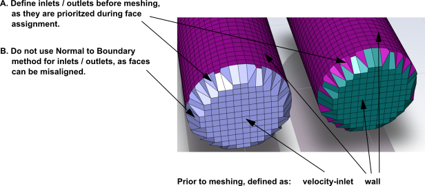
The surface area of a boundary generated by the Rapid Octree mesher may not exactly match that of the original geometry. You can minimize this discrepancy by assigning boundary types to the surfaces prior to using the Rapid Octree mesher, as inlets and outlets will be prioritized when assigning individual cell faces to the boundary zones in order to best preserve the projected area (see note A. in the following figure). It is recommended that you evaluate the surface areas of inlets and outlets after mesh generation, and if they are not appropriate, perform the mesh generation from the geometry again using settings that will produce a more refined mesh.
Cell faces at the edges of inlets and outlets may not be oriented with the original geometry surface, and so when defining the boundary conditions for such zones in the solution mode it is recommended that you do not use the Normal to Boundary specification method for the velocity or direction. See note B. in the following figure.
If you cannot avoid the defeaturing by these steps, then you could instead try enabling the Improve Geometry Resolution option, as described in Improve Geometry Resolution.
You can only have constant boundary cell sizes when using the Cartesian Snapping boundary treatment method.
With the Cartesian Snapping boundary treatment method, the boundary geometry must be a consistently closed triangulated surface (that is, there should be no gaps, no overlaps, no self-intersection, no interior boundary zones bounding mesh volumes on both sides) with consistent normals. With the Boundary Projection boundary treatment method, it may be possible for small faults to be tolerated.
Multiple cell zones can only be created using the Selected Material Points or All Volumetric Regions selection from the Volume Specification drop-down list.
To ensure an acceptable mesh quality for the projection boundary handling, nodes may be moved away from the boundary, which results in small bumps in the surface mesh. This occurs mostly with very coarse meshes, at sharp corners, and at mesh size changes. Using a higher volume transition exponent and/or mesh refinement can mitigate the effect.