


An essential point in the implementation of turbulence models is the near-wall treatment.
There are two distinct branches for setting the wall boundary conditions depending on first near
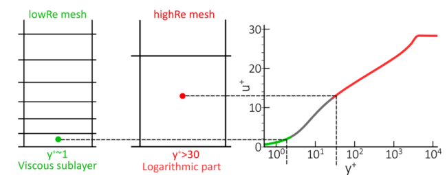
wall grid step (see Figure 4.17: Computational meshes for low and high Reynolds number cases). The first constitutes a low Reynolds
number formulation (lowRe) where the first near wall grid step is inside the viscous sublayer of
the boundary layer ( < 5). The second corresponds to high Reynolds number (highRe) meshes where
wall functions are activated. In this case, the first near wall grid step corresponds to the
logarithmic profile ( > 30). Between these two cases, the so-called buffer layer is located.
Ideally simulations should be computed with meshes where is 1 , however this requirement is not always easy to achieve, especially in
industrial computations at high Reynolds numbers and with complex geometries. It is also not
always possible to create pure wall function meshes with > 30 on the entire geometry. Wall-formulations have therefore been developed
which smoothly blend between the two limits. Such formulations are termed "-insensitive near-wall treatment".
< 5). The second corresponds to high Reynolds number (highRe) meshes where
wall functions are activated. In this case, the first near wall grid step corresponds to the
logarithmic profile ( > 30). Between these two cases, the so-called buffer layer is located.
Ideally simulations should be computed with meshes where is 1 , however this requirement is not always easy to achieve, especially in
industrial computations at high Reynolds numbers and with complex geometries. It is also not
always possible to create pure wall function meshes with > 30 on the entire geometry. Wall-formulations have therefore been developed
which smoothly blend between the two limits. Such formulations are termed "-insensitive near-wall treatment".
As the formulation suggests, these methods are not entirely "-insensitive" and a small difference in wall shear stress values is typically
observed in the buffer layer, compared to the reference fine grid solution.
The goal of the -insensitive near-wall treatment is to minimize these variations and to develop
wall boundary conditions which allow for solutions to be as insensitive to near-wall mesh
resolution as possible for the wall shear stress and wall heat flux assuming a sufficient overall
resolution of the boundary layer.
In turbulence models based on the ω-equation, the wall shears stress is controlled by
the values specified for ω at the wall. In Ansys Fluent, two -insensitive near-wall treatments are available:
correlation: blends between analytical expressions of the viscous sublayer and logarithmic region depending on (default).tabulated: employs a table look-up for the wall value of ω to minimize analytical interpolation errors between the two regimes.
Both formulations were calibrated using fully developed plane Couette flow and will be outlined in the following sections. Beside the treatment of wall ω other quantities also require a gradual shift from wall functions to a low-Re formulation when the mesh is refined.
The wall shear stress  is needed as a boundary condition and calculated in the following way:
 | (4–389) |
where  denotes the density. Equation 4–389 is based on the
friction velocity
denotes the density. Equation 4–389 is based on the
friction velocity  and the alternative velocity scale
  , which has been introduced to improve the behavior at separation. Both
quantities are blended between the viscous sublayer and the logarithmic region.
, which has been introduced to improve the behavior at separation. Both
quantities are blended between the viscous sublayer and the logarithmic region.
The friction velocity  is given by:
 | (4–390) |
where
 | (4–391) |
 | (4–392) |
with  =0.4187 and E=9.793.
  represents the mean velocity tangent to the wall at the wall-adjacent cell
centroid. The non-dimensional distance from the wall is defined using
represents the mean velocity tangent to the wall at the wall-adjacent cell
centroid. The non-dimensional distance from the wall is defined using  :
:
 | (4–393) |
 denotes the distance from the wall at the wall-adjacent cell centroid and
  the molecular viscosity.
For the blending of the alternative velocity scale  the following formulation is used:
 | (4–394) |
where k denotes the turbulence kinetic energy at the wall-adjacent cell centroid.
For the transport equation of the turbulence kinetic energy, a zero flux boundary condition
is specified not only in the logarithmic region, but also (artificially) for the integration
down to the wall. The wall production term is blended between the viscous sublayer and
logarithmic region. The production term can be written using  and
and  in the following way:
 | (4–395) |
which gives the following relations for the viscous sublayer and logarithmic region:
 | (4–396) |
 | (4–397) |
Note that  is not based on a gradient computation, but directly derived from the log-law
relation in Equation 4–392.
is not based on a gradient computation, but directly derived from the log-law
relation in Equation 4–392.
The blended form of the wall production term finally reads:
 | (4–398) |
In the transport equation of the specific dissipation rate, the value of ω at the wall is prescribed. The wall value is blended between the relations of the viscous sublayer and logarithmic region in the following way:
 | (4–399) |
where  and
and  denote the density and the dynamic viscosity, respectively. u* represents the
alternative velocity scale given in Equation 4–394.
denote the density and the dynamic viscosity, respectively. u* represents the
alternative velocity scale given in Equation 4–394.
Analytical solutions for  can be given for both the laminar sublayer and the logarithmic region. This
strategy can used to define a
can be given for both the laminar sublayer and the logarithmic region. This
strategy can used to define a  -insensitive near wall treatment by blending between these two analytical
expressions depending on
-insensitive near wall treatment by blending between these two analytical
expressions depending on  :
:
 | (4–400) |
 | (4–401) |
 | (4–402) |
This formulation is the current default treatment in Ansys Fluent and is labelled further-on as
"correlation". Incompressible plane Couette flow at Reynolds number
106 has been used to calibrate the entire formulation for momentum
and turbulence equations in order to minimize the variation of the wall shear stress over  . This leads to a value of 1/3 for Ccalib and 1.3 for
Cexp. However, due to its analytical expression, this formulation offers
only limited possibilities for fine tuning.
. This leads to a value of 1/3 for Ccalib and 1.3 for
Cexp. However, due to its analytical expression, this formulation offers
only limited possibilities for fine tuning.
A further improvement was achieved by using a table look-up for  for a wide range of
  values. Incompressible plane Couette flow has again been used to calibrate
this formulation in order to minimize the variation of the wall shear stress over
values. Incompressible plane Couette flow has again been used to calibrate
this formulation in order to minimize the variation of the wall shear stress over  . For this purpose, a fine grid solution was created, and the resulting wall
shear stress was used as a reference on coarser grids. A table was created by running the plane
Couette flow for various meshes, storing the optimal
. For this purpose, a fine grid solution was created, and the resulting wall
shear stress was used as a reference on coarser grids. A table was created by running the plane
Couette flow for various meshes, storing the optimal  and then transforming the obtained data sets into an efficient table look-up
for
and then transforming the obtained data sets into an efficient table look-up
for  .
.
Specific tables have been created for BSL, SST, and GEKO turbulence models and this method
is further-on labelled as "tabulated". All other ω-based
turbulence models are using the SST table look-up so that for example, the Transition SST,
DES-SST, and SAS-SST (all implemented as separate models) are using a consistent table.
Both formulations agree well for high quality meshes with small values of y+ (y+ < 1) and moderate expansion ratios. Although these meshes are generally recommended, it might not always be possible to create such meshes due to the complexity of the applications. The table look-up offers a more accurate prediction of the wall shear stress, especially for poorer meshes having larger values of y+ and/or higher expansion ratios.
As an example of this improvement, the results of a zero pressure gradient flat plate boundary layer flow are presented below. The setup is based on the experiment of Wieghardt & Tillmann [783] and the Reynolds number based on inlet velocity and length of the flat plate is Re=107. Figure 4.18: Comparison of the skin friction distribution on a fine (y+ ~ 0.1, left) and coarse (y+ ~ 22, right) mesh for the ‘correlation’ and ‘tabulated’ near wall treatments with SST. shows the skin friction distribution for a fine (y+ ~ 0.1) and coarse (y+ ~ 22) mesh computed with the SST turbulence model. The visual difference between the 2 formulations appears small and confirms that the correlation model is already reasonably close.
Figure 4.18: Comparison of the skin friction distribution on a fine (y+ ~ 0.1, left) and coarse (y+ ~ 22, right) mesh for the ‘correlation’ and ‘tabulated’ near wall treatments with SST.
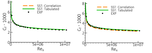
However, looking at the overall drag reveals that the "tabulated" (new) model is superior for this case. The error in drag prediction is defined as
 | (4–403) |
where the reference solution  corresponds to the solution on a very fine mesh with y+ ~ 0.001. The results
are summarized in Table 1 and it can be seen that the error is strongly reduced on the coarse
mesh for the "tabulated" near wall treatment:
corresponds to the solution on a very fine mesh with y+ ~ 0.001. The results
are summarized in Table 1 and it can be seen that the error is strongly reduced on the coarse
mesh for the "tabulated" near wall treatment:
Table 4.3: Error in drag prediction on a fine (y+ ~ 0.1) and coarse mesh (y+ ~ 22) for the ‘correlation’ and ‘tabulated’ near wall treatments with SST, relative to (y+ ~ 0.001) mesh
|
Mesh |
| |
|---|---|---|
|
SST: correlation |
SST: tabulated | |
|
y+ ~ 0.1 |
0.47% |
0.05% |
|
y+ ~ 22 |
5.86% |
0.02% |

The near wall treatment of the energy equation follows a Kader blending method between the viscous sublayer and logarithmic law of the wall as outlined by Equation 4–379.
For the
tabulatedoption, there are specially calibrated tables for BSL, SST, and GEKO. All other omega-based turbulence models are using the SST table look-up so that for example, the Transition SST, DES-SST and SAS-SST (all implemented as separate models) are using a consistent table look-up.Both the formulations can also be combined with the Standard Roughness Model.
Note: Note: The High Roughness (Icing) Model only works on y+ ~ 1 meshes and uses a separate near wall treatment for the walls where it is specified.