


The following ease of use features are available when defining joints:
Renaming Joint Objects Based on Definition
When joints are created, Mechanical automatically names each of the joint objects with a name that includes the type of joint followed by the names of the joined parts included as child objects under the Geometry object folder. For example, if a revolute joint connects a part named ARM to a part named ARM_HOUSING, then the object name becomes Revolute - ARM To ARM_HOUSING.
The automatic naming based on the joint type and geometry definition is by default. You can however change the default from the automatic naming to a generic naming of Joint, Joint 2, Joint 3, and so on by opening the dialog and setting Auto Rename Connections to No under the Connections group.
If you then want to rename any joint object based on the definition, click the right mouse button on the object and choose Rename Based on Definition from the context menu. You can rename all joints by clicking the right mouse button on the Joints folder then choosing Rename Based on Definition. The behavior of this feature is very similar to renaming manually created contact regions. See Renaming Contact Regions Based on Geometry Names for further details including an animated demonstration.
Remote Connection Display
When defined as a , joints are considered to be a remote boundary condition, and can make use of remote points that were either specifically defined or created internally by the application. To do a visual check, you can display the connection lines between your scoping and the remote point by selecting the Remote Point Connections option of the Style group (Display tab). An example is illustrated here of a spring scoped to two edges.
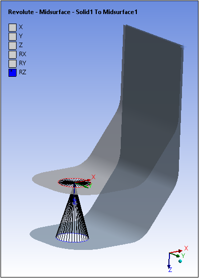
Joint Legend
When you highlight a joint object, the accompanying display in the Geometry window includes a legend that depicts the free degrees of freedom characteristic of the type of joint. A color scheme is used to associate the free degrees of freedom with each of the axis of the joint's coordinate system shown in the graphic. An example legend is shown below for a slot joint.
You can display or remove the joint legend using from the main menu.
Disable/Enable Transparency
The Enable Transparency feature enables you to graphically highlight a particular joint that is within a group of other joints, by rendering the other joints as transparent. The following example shows the same joint group presented in the Joint Legend section above but with transparency enabled. Note that the slot joint alone is highlighted.
To enable transparency for a joint object, click the right mouse button on the object and choose Enable Transparency from the context menu. Conversely, to disable transparency, click the right mouse button on the object and choose Disable Transparency from the context menu. The behavior of this feature is very similar to using transparency for highlighting contact regions. See Controlling Transparency for Contact Regions for further details including an animated demonstration.
Hide All Other Bodies
You can hide all bodies except those associated with a particular joint.
To use this feature, click the right mouse button on the object and choose from the context menu. Conversely, to show all bodies that may have been hidden, click the right mouse button on the object and choose from the context menu.
Flip Reference/Mobile
For body-to-body joint scoping, you can reverse the scoping between the Reference and Mobile sides in one action. To use this feature, click the right mouse button on the object and choose Flip Reference/Mobile from the context menu. The change is reflected in the Details view of the joint object as well as in the color coding of the scoped entity on the joint graphic. The behavior of this feature is very similar to the Flip Contact/Target feature used for contact regions. See Flipping Contact and Target Scope Settings for further details including an animated demonstration.
Joint DOF Checker
Once joints are created, fully defined, and applied to the model, a Joint DOF Checker calculates the total number of free degrees of freedom. The number of free degrees of freedom should be greater than zero in order to produce an expected result. If this number is less than 1, a warning message is displayed stating that the model may possibly be overconstrained, along with a suggestion to check the model closely and remove any redundant joint constraints.
To display the Joint DOF Checker information, highlight the Connections object and click the Worksheet button. The Joint DOF Checker information is located just above the Joint Information heading in the worksheet.
Redundancy Analysis
This feature enables you to analyze an assembly held together by joints. This analysis will also help you to solve over constrained assemblies. Each body in an assembly has a limited degree of freedom set. The joint constraints must be consistent to the motion of each body, otherwise the assembly can be locked, or the bodies may move in unwanted directions. The redundancy analysis checks the joints you define and indicates the joints that over constrain the assembly. To analyze an assembly for joint redundancies:
Right-click the Connections object, and then select Redundancy Analysis to open a worksheet with a list of joints.
Click to perform a redundancy analysis. All the over constrained joints are indicated as redundant.
Click the Redundant label, and then select or to resolve the conflict manually.
or
Click Convert Redundancies to Free to remove all over constrained degrees of freedom.
Click to update the joint definitions.
Note: Click Export to save the worksheet to an Excel/text file.
Important: When a model contains a Point On Curve joint, the Configure and Assemble options are disabled for all the joints. This is also the case for a redundancy analysis that includes a Point On Curve joint.
Model Topology
The Model Topology worksheet provides a summary of the joint connections between bodies in the model. This feature is a convenient way of verifying and troubleshooting a complex model that has many parts and joints. The Model Topology worksheet displays the connections each body has to other bodies, and the joint through which these bodies are connected. Additional information for the joints is provided, including the joint type and the joint representation for the rigid body solver (i.e. whether the joint is based on degrees of freedom or constraint equations).
To display the model topology, right-click the Connections object, and then select . The worksheet displays in the Data View. The content of the worksheet can be exported as a text file using the button.
Joints based on degrees of freedom are labeled either Direct or Revert in the Joint Direction column of the Model Topology table. Direct joints have their reference coordinate system on the ground side of the topology tree. Revert joints have their mobile coordinate system on the ground side. This information is useful for all post-processing based on python scripting, where internal data can be retrieved. For reverted joints, some of the joint internal results need to be multiplied by -1.
Refer to the Ansys Rigid Dynamics Theory Manual for more information on model topology and selecting degrees of freedom.