


- Constrained degrees of freedom:
None
- Example:
A Bushing has six degrees of freedom, three translations and three rotations, all of which can potentially be characterized by their rotational and translational degrees of freedom as being free or constrained by stiffness.
For a Bushing, the rotational degrees of freedom are defined as follows:
The first is a rotation around the reference coordinate system X Axis.
The second is a rotation around the Y Axis after the first rotation is applied.
The third is a rotation around the Z Axis after the first and second rotations are applied.
The three translations and the three rotations form a set of six degrees of freedom. In addition, the bushing behaves, by design, as an imperfect joint, that is, some forces developed in the joint oppose the motion.
The three translational degrees of freedom expressed in the reference coordinate system and the three rotations are expressed as: Ux, Uy, Uz, and Ψ, Θ, φ. The relative velocities in the reference coordinate system are expressed as: Vx, Vy, and Vz. The three components of the relative rotational velocity are expressed as: Ωx, Ωy, and Ωz. Note that these values are not the time derivatives of [Ψ, Θ, φ]. They are a linear combination.
The Bushing joint includes a Formulation property that enables you to specify a desired element type. The Formulation property options include (Multi-Point Constraint) and . The option uses the MPC184 element and the option uses the COMBI250 element.
Important: The option is only supported for the following analysis types:
All Substructure analyses when the Joint as included in the Condensed Part.
Modal and Harmonic Response.
Static Structural when you active Beta Options.
For the MPC Formulation, the degrees of freedom are expressed in the reference coordinate system as discussed above. The same holds true for the Bushing Formulation, however, it uses an element coordinate system as specified by an associated property. This Element Coordinate System property is set to the by default. As desired, you can define an element coordinate system manually.
The forces developed in the Bushing are expressed as:
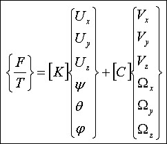
Where:
[F] is force and [T] is Torque, and [K] and [C] are 6x6 matrices (defined using Stiffness Coefficients and Dampening Coefficients options). Off diagonal terms in the matrix are coupling terms between the DOFs.
You can use these joints to introduce flexibility to an over-constrained mechanism. Note that very high stiffness terms introduce high frequencies into the system and may penalize the solution time when using the Ansys Rigid Dynamics solver. If you want to suppress motion in one direction entirely, it is more efficient to use Joint DOF Zero Value Conventions instead of a very high stiffness.
Application
To add a bushing:
Select the Connections object in the tree and select Bushing from either the Body-Groundor Body-Body drop-down menus on the Connections Context Tab. By default, the Worksheet displays.
Matrix data for the Stiffness Coefficients and Dampening Coefficients is entered in the Worksheet.
Note:For an MPC Formulation, entries are based on a Full Symmetric matrix. For a Bushing Formulation, only diagonal entries are available to define.
You can change the default display setting of the Worksheet using the Bushing Joint Worksheet View property in the Connections category of the Options dialog. Set the property to .
As needed, specify a desired element type using the Formulation property.
When you specify the option, the Element Coordinate System property also displays. As needed, specify a user-defined coordinate system. The default setting for this property is .
Select the Graphics tab. Based on whether your bushing is Body-Ground or Body-Body, scope the bushing to geometry.
You can scope a bushing to single or multiple faces, single or multiple edges, or to a single vertex. Body-Body scoping requires Reference and Mobile scoping. The scoping for the Reference and Mobile sides of the joint cannot be the same.
Body-Ground assumes that the Reference is grounded (fixed). Only the Mobile side requires scoping.
Specified the various additional properties as needed for your analysis, that may include:
Coordinate System
Behavior
Pinball Region
See the Joint Properties section for specific property information.
Non-Linear Force-Deflection Curve
You can use a nonlinear force-deflection curve to simulate a multi-rate bushing with nonlinear stiffness. In Mechanical, you can accomplish this using a linear piecewise curve. You can use this calculation when defining Condensed Parts and using the MPC Formulation (only).
Note: The Ansys Explicit Dynamics solver does not support Tabular Data entry.
To define a nonlinear Force-Deflection curve:
In the Worksheet, select the cell in which you want to define a non-linear force-deflection curve.
Right-click the cell and then select .
Enter Displacement and Force (or Angle and Moment) values (minimum of two rows of data) in the Tabular Data window. The application plots your entries in the Graph window.
Note: If tabular entries exist in the stiffness matrix, the Mechanical APDL solver does not account for constant terms and non-diagonal (coupled) terms.
Samcef Solver Comment Object
BUSHING