


The details of your simulation setup depend on the type of template you have chosen, however, you can use the Outline View or the Ribbon to progress through the setup process. For instance, set your general simulation properties, followed by material properties, cell zone properties, boundary condition properties, and solution properties, etc.
General properties: allow you to define the overall simulation. Here, you can view and adjust any geometry, mesh, or calculation settings, as well as assorted physics options. See General Simulation Settings or more information.
Material properties: allow you to define the chemical and physical properties of a substance in your simulation. See Materials or more information.
Cell Zone properties: allow you to categorize various portions of your geometry (mesh). See Cell Zones or more information.
Boundary Condition properties: allow you to define the physical conditions at specific boundaries in your simulation, depending on the type of simulation you are setting up. See Boundary Conditions or more information.
If temperature changes are being considered, Thermal Conditions can also be associated at boundaries.
Assign Pressures properties: (optional) allows you to set the pressure level for a fluid flow simulation within a closed domain. See Pressure Assignment or more information.
Mesh Deformations properties: (optional) allow you to define how the mesh deforms in your simulation. See Mesh Deformations for more information.
Adaptive Meshing properties: (optional) allow you to define how the mesh can be adapted as it changes during your simulation. See Adaptive Meshing for more information.
Use the General node to access general properties of the selected simulation (Figure 4.55: General Simulation Properties).
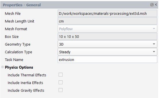
Here, most of the fields are informational, however, you can go to this page to change the Geometry Type (that depends on the loaded mesh), Calculation Type, Task Name, or any of the Physics Options.
By default, the Calculation Type is Steady, however, you may change this and select among Continuation (useful for specific non-linear calculations), Transient and Volume of fluid. In both of the latter cases, you are prompted for the Duration of the simulation.
Among the general physical options, you may decide to incorporate thermal effects, fluid inertia, and/or gravity effects; in the latter case, the components of the gravity vector must be given.
Use the Materials node to access materials and their properties of the selected simulation (Figure 4.56: Material Properties).
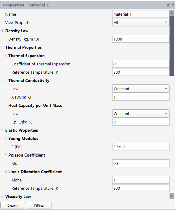
Here, you can change the Name and elect to view and edit all (or a selection) of the material properties (such as viscoelastic and/or thermal properties) using the View Properties field.
Use the New... button (available in the property page when no material has yet been created, or when using the context menu, or in the Setup portion of the ribbon) to create a new object with its own unique properties. Assign a name and other assorted properties to the new material.
Use the Import from library button to open the Library of Materials dialog. Here, you can choose a material Family, and a corresponding Material to use in your simulation.
Use the Import from file button to browse for and select a separate materials library file and add it to your simulation. Browse to the location in the Fluent Materials Processing installation where relevant material data can be found. For example:
C:\Program Files\ANSYS
                        Inc\v242\polyflow\polyflow24.2.0\Material_Data\
Various subdirectories therein contain materials defined using the
.mprmatformat that is compatible with the Fluent Materials Processing workspace.Use the Export button to save a material definition to a separate file using the
.mprmatformat.Use the Fitting button to open Fluent Materials Processing where you can perform a fitting of your material data.
If you have not already done so, you are required to assign a fluid model to your material fitting using the Define Fluid Model dialog.
Options include:
For more information, see Material Properties in the Polyflow User's Guide.
See Simplified Viscoelastic Law Properties for details.
For more information, see Simplified Viscoelastic Model in the Polyflow User's Guide.
The differential approach to modeling viscoelastic model is appropriate for most practical applications. Many of the most common models for viscoelastic model are provided in Fluent Materials Processing, including
Maxwell (see Upper-Convected Maxwell Model in the Polyflow User's Guide)
Oldroyd-B (see Oldroyd-B Model in the Polyflow User's Guide)
Giesekus (see Giesekus Model in the Polyflow User's Guide)
Phan Thien-Tanner (see Phan-Thien-Tanner Model in the Polyflow User's Guide)
Fene-P (see FENE-P Model in the Polyflow User's Guide)
POMPOM (see POM-POM Model [DCPP] in the Polyflow User's Guide)
Leonov (see Leonov Model in the Polyflow User's Guide)
Appropriate choices for the viscoelastic model and related parameters can yield qualitatively and quantitatively accurate representations of viscoelastic behavior.
For the Number of Relaxation Modes, when a multi-mode viscoelastic model is used, the total extra-stress tensor is decomposed into a sum of individual viscoelastic components, and one purely viscous component.
As for Thermal Dependencies, the viscosity in a thermal differential viscoelastic model can be temperature-dependent. For thermal differential viscoelastic models, the relaxation time is multiplied by the same temperature shift function. Temperature-dependent functions available for thermal differential viscoelastic models are as follows, described in Theory and Equations in the Polyflow User's Guide:
None
Approximate Arrhenius
Arrhenius
WLF
See Differential Viscoelastic Law Properties for details, or for more information, see Theory and Equations Extra-Stress Tensor, and Differential Viscoelastic Models in the Polyflow User's Guide.
For shell models, a multi-mode integral viscoelastic model for blow molding or thermoforming applications can be used. This method makes use of a membrane element.
See Integral Viscoelastic Law Properties for details.
For more information, see 3D Viscoelastic Blow Molding Simulations in the Polyflow User's Guide.
See Reinforcement Properties for details.
For more information, see Orthotropic Materials in the Polyflow User's Guide.
For simulations that need to model physical foaming, such as in the inverse die lip shape prediction for the extrusion of foamed profiles. In such cases, gas is dissolved in the polymer and the gas bubbles begin to expand as soon as the polymer leaves the die.
See Foaming Properties for details.
Note: The following limitations are known for the Fluent Materials Processing workspace:
Foaming cannot be combined with multiple materials and/or transport of species and/or generalized expressions defined on material properties.
If an expression is defined on density, you cannot impose a mass flow rate at the inlets and/or the outlets.
See Viscosity Law in Porous Medium Properties for details.
For more information, see Theory in the Polyflow User's Guide.
Use the Species node within the Materials group box to define the transport of species for your simulation.
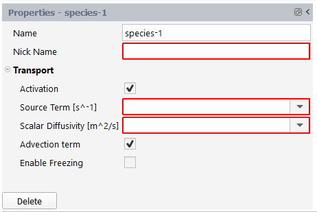
Here you can define up to 6 species and change the Name and Nick Name of the defined species if necessary. Clicking on Activation makes the workspace define a transport model for the current species, and model for which necessary parameters will be requested. The support of the model is the union of fluid zones. The equation for modeling species transport in the Fluent Materials Processing workspace is as follows:
 | (4–8) |
where the Source Term and Scalar
Diffusivity represent  and
and  , respectively. The Advection term option can
be disabled if you do not want to take the affects of
, respectively. The Advection term option can
be disabled if you do not want to take the affects of  into account. Note that
  is always equal to
 1. The
Enable Freezing option can be turned on if you want to freeze
the transported species on a part of the computational domain. Although the
Source Term is displayed with [1/s]
unit in the species properties panel, species transport can be defined using
variables with units as well. For example, if the transport of temperature
[K] is specified for the source term, the resulting source
term will have units of [K/s], despite the properties panel
displaying units of [1/s].
Use the Cell Zones node to access cell zone definitions for your simulation. Cell zones represent the domain of your simulation.
Use the New... button to create a new cell zone object with its own unique properties. Depending on the type of simulation you are setting up, cell zones can be one of the following types:
Fluid
Solid
Porous media
Fixed mold (transient simulations only)
Moving mold (transient simulations only)
Restrictor part
Moving part
Use the Display button to show an existing cell zone in the graphics window.
Use the Delete button to remove an existing cell zone
When the Type is set to Fluid, use the Cell Zones node to access fluid cell zone definitions for your simulation (Figure 4.58: Fluid Cell Zone Properties).
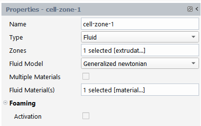
Here, you can change the Name, assign Zones, and change the Fluid Model for the fluid zone (such as Generalized Newtonian, Simplified viscoelastic, Differential viscoelastic, or Integral viscoelastic), and/or whether your simulation involves coextrusion (that is, involving Multiple Materials).
Typically, you define a fluid zone when you need to simulate the flow of a material, such as flow in a die, a free extrudate, a pressing process, coextrusion, blow molding, thermoforming, and so on.
See Fluid Cell Zone Properties for details.
For more information, see Generalized Newtonian Flow and Viscoelastic Flows in the Polyflow User's Guide.
When the Type is set to Solid, use the Cell Zones node to access solid cell zone definitions for your simulation (Figure 4.59: Solid Cell Zone Properties).
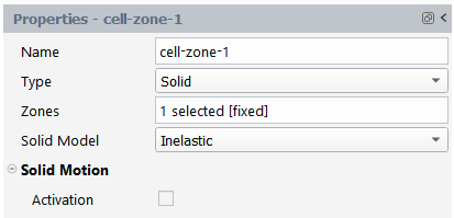
Here, you would typically set the Name, select the appropriate Zones, set the Solid Model as either Elastic or Inelastic, and assorted Solid Deformation properties, if applicable.
Typically, you define a solid zone when you need to simulate fluid-structure interaction (FSI) or simulate heat conduction in a solid. For an FSI simulation, Elastic must be selected for the Solid Model and a fluid-solid interface must be defined if the solid is connected to a fluid region as outlined in Fluid-Solid Interface Boundary Conditions.
See Solid Cell Zone Properties for details.
When the Type is set to Porous media, use the Cell Zones node to access porous cell zone definitions for your simulation (Figure 4.60: Porous Media Cell Zone Properties).
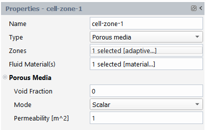
Here, you would typically set the Name, select the appropriate Zones, Fluid Materials, and assorted Porous Media properties. If thermal effects are taken into account, the Fluid Material(s) and the Solid Material are required.
See Porous Cell Zone Properties for details.
For more information, see Porous Media in the Polyflow User's Guide.
When the Type is set to Fixed mold, use the Cell Zones node to access fixed mold cell zone definitions for your simulation (Figure 4.61: Fixed Mold Cell Zone Properties).
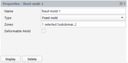
Here, you would typically set the Name, select the appropriate Zones, and if applicable, specify the fixed mold as a Deformable Mold. If thermal effects are taken into account, it is necessary to specify the Mold Model (Adiabatic, Fixed temperature or Heat conduction). For a fixed mold that accounts for thermal effects or mold deformation (Deformable Mold option enabled), a Solid Material must be defined. Note that the Deformable Mold option and the Heat conduction Mold Model are not supported for 2D shell geometries.
Typically, you define a fixed mold zone when you need to simulate contact between a fluid and a fixed solid. The thermal impact of contact can also be taken into account.
When the Type is set to Moving mold, use the Cell Zones node to access moving mold cell zone definitions for your simulation (Figure 4.62: Moving Mold Cell Zone Properties).
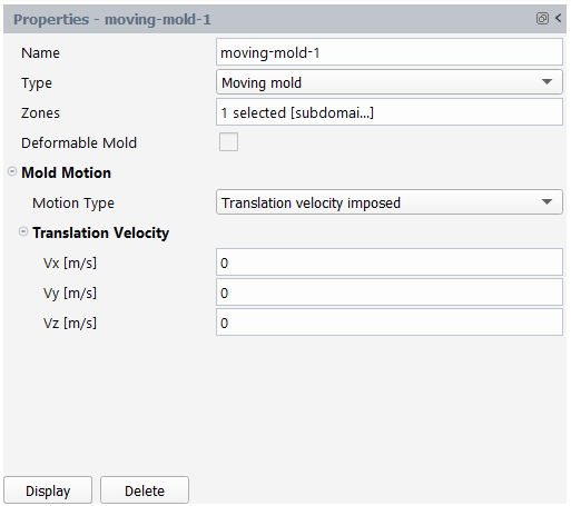
Here, you would typically set the Name, select the appropriate Zones, specify the moving mold as a Deformable Mold if applicable, and define the Mold Motion properties for the moving mold. If thermal effects are taken into account, it is necessary to specify the Mold Model (Adiabatic, Fixed temperature or Heat conduction). Note that the Deformable Mold option and the Heat conduction Mold Model are not supported for 2D shell geometries.
Next, you have to specify the Motion Type, the Motion Type can be either Translation velocity imposed, Translation force imposed or General velocity driven motion. Depending on the selection for the motion type, you are prompted for additional parameters, such as velocity components, force components, mass of mold, limit of mold displacement, etc.
Typically, you define a moving mold zone when you need to simulate contact between a fluid and a moving solid. Mold deformation or the thermal impact of contact can also be taken into account.
Allows you to set mesh superposition options for restrictor part cell zones in your simulation.
A restrictor is an obstacle placed in the flow channel to better control the pressure drop and/or the flow balance. Taking advantage of the Mesh Superposition Technique allows you to easily experiment and optimize the size and location of the restrictor.
When the Type is set to Restrictor part, use the Cell Zones node to access restrictor cell zone definitions for your simulation (Figure 4.63: Restrictor Cell Zone Properties).
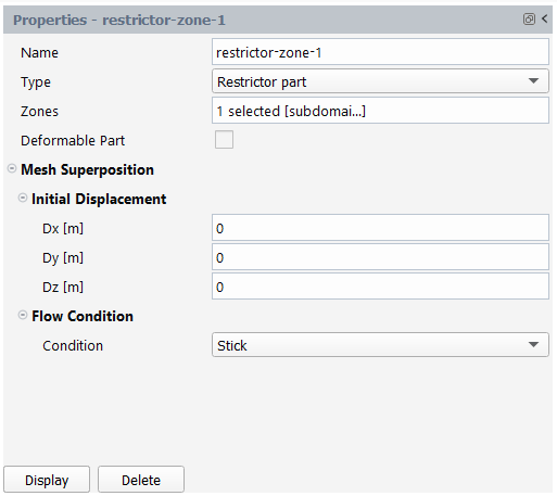
Here, you would typically set the Name, select the appropriate Zones, specify the restrictor as a Deformable Part if applicable, and define the assorted Mesh Superposition properties for the restrictor. When the restrictor is defined as a deformable part, or if thermal effects are taken into account, it is necessary to specify a Solid Material for the restrictor part.
See Restrictor Zone Properties for more details.
For more information, see Flows with Internal Moving Parts in the Polyflow User's Guide.
Allows you to set mesh superposition properties on any moving part cell zones in your simulation.
A moving part represents a moving solid part such as the rotating screw in an extruder, an impeller in a mixing device, a piston in an injection machine, etc.
When the Type is set to Moving part, use the Cell Zones node to access moving part cell zone definitions for your simulation (Figure 4.64: Moving Part Cell Zone Properties).
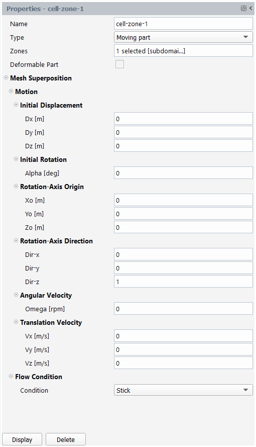
Here, you would typically set the Name, select the appropriate Zones, specify the moving part as a Deformable Part if applicable, and define the assorted Mesh Superposition properties for the moving part. When the moving part is defined as a deformable part, or if thermal effects are taken into account, it is necessary to specify a Solid Material for the moving part.
See Moving Part Zone Properties for details.
For more information, see Flows with Internal Moving Parts in the Polyflow User's Guide.
This section describes the various boundary conditions available in the Fluent Materials Processing workspace. If temperature changes are being considered, then there can be Thermal Conditions associated at the boundaries as well.
Use the New... button to create a new boundary condition object with its own unique properties. Depending on the type of simulation you are setting up, boundary conditions can be one of the following types:
Inflow
Outflow
Wall
Symmetry
Free surface
Extrudate exit
Vent
Zero velocity
Zero force
Porous wall
etc.
The following sections describe the boundary conditions in more detail:
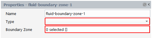
Specify conditions for the fluid material(s) and, if applicable, their thermal conditions at the various boundaries in your simulation (Figure 4.65: Fluid Boundary Properties).
- 4.8.5.1.1. Inflow Fluid Boundary
- 4.8.5.1.2. Outflow Fluid Boundary
- 4.8.5.1.3. Wall Fluid Boundary
- 4.8.5.1.4. Symmetry Fluid Boundary
- 4.8.5.1.5. Free Surface Fluid Boundary
- 4.8.5.1.6. Extrudate Exit Fluid Boundary
- 4.8.5.1.7. Vent Fluid Boundary
- 4.8.5.1.8. Zero Velocity Fluid Boundary
- 4.8.5.1.9. Zero Force Fluid Boundary
- 4.8.5.1.10. Porous Wall Fluid Boundary
- 4.8.5.1.11. Force Fluid Boundary
- 4.8.5.1.12. Thermal Conditions for Fluid Boundaries
- 4.8.5.1.13. Species Conditions for Fluid Boundaries
Inlets define conditions where flow is expected to enter the solution domain.
When the Type is set to Inflow, use the Fluid Boundary Zone node to access inflow boundary definitions for your simulation (Figure 4.66: Inflow Fluid Boundary Properties).
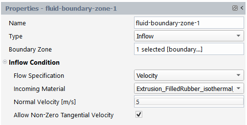
Here, you would typically set the Name, select the appropriate Boundary Zone, and assorted Inflow Condition properties for the inflow fluid boundary. There are several ways of defining an inflow boundary condition. You can:
Impose a volume or mass flow rate, and the solver will calculate the corresponding velocity profile on the basis of the flow rate, the rheology and the geometry of the inlet. Here, you can also specify whether this calculation is performed before or in conjunction with the main simulation, or simply leave the choice to the solver. Note that imposing a flow rate is the recommended choice for viscoelastic models.
Assign a constant normal velocity value, possibly combined with a free or a zero tangential velocity component.
Read a profile using a CSV file.
See Inflow Fluid Boundary Properties for more details.
For additional information, see Inflow Condition, Inflow Calculation for Generalized Newtonian Flow, and Inflow Calculation for Viscoelastic Flow in the Polyflow User's Guide.
Outlets define conditions where flow is expected to leave the solution domain.
When the Type is set to Outflow, use the Fluid Boundary Zone node to access outflow boundary definitions for your simulation (Figure 4.67: Outflow Fluid Boundary Properties).
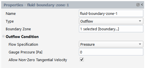
Here, you would typically set the Name, select the appropriate Boundary Zone, and assorted Outflow Condition properties for the outflow fluid boundary. There are several ways to define an outflow boundary condition. You can:
Assign an exit pressure on the selected outlet.
Impose a volume or mass flow rate, and the solver will calculate the corresponding velocity profile on the basis of the flow rate, the rheology and the geometry of the outlet. Here, you can also specify whether this calculation is performed before or in conjunction with the main simulation, or simply leave the choice to the solver. Note that imposing an exit flow rate is often a recommended choice for viscoelastic models within a die.
Assign a constant normal velocity value.
In each case, you can specify whether the resulting normal velocity profile is combined with a free or a zero tangential velocity component.
In addition, you can also read a pre-defined velocity profile using a CSV file.
For polymer extrusion simulations, when the outlet represents an actual exit from which the fluid can freely flow, tangential velocities at the outlet could be allowed (such as a die exit). However, when the outlet is at the end of the computation domain, but not at the end of the channel in which the fluid flows, tangential velocities at outlets should preferably not be allowed because the fluid is still confined after the outlet.
See Outflow Fluid Boundary Properties for more details.
For additional information, see Outflow Condition, Outflow Condition for Generalized Newtonian Flow, and Outflow Condition for Viscoelastic Flow in the Polyflow User's Guide.
Wall boundaries assigned to surfaces of a fluid region prevent flow through those surfaces. The conditions that best describe the forces applied to a wall are summarized below.
When the Type is set to Wall, use the Fluid Boundary Zone node to access wall boundary definitions for your simulation (Figure 4.68: Wall Fluid Boundary Properties).
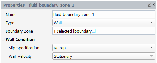
Here, you would typically set the Name, select the appropriate Boundary Zone, and assorted Wall Condition properties for the wall fluid boundary.
The Slip Specification includes the following options:
No slip: the fluid sticks to the wall. If the wall is moving, the fluid moves with the same velocity as the wall. For additional information, see Zero Wall Velocity Condition in the Polyflow User's Guide.
Partial slip: the fluid partially slips to the wall, that is, the relative velocity between the fluid and the wall is a function of the tangential stress at the wall. Several slipping functions are available: Navier’s law, generalized Navier’s law, threshold and generalized threshold laws, and an asymptotic law where the growth of the tangential stress versus the tangential velocity is asymptotically bounded to a given value. For additional information, see Slip Condition in the Polyflow User's Guide.
Free slip: a frictionless wall. For additional information, see Slip Condition in the Polyflow User's Guide. Also, for additional information about the wall velocity, see Cartesian Velocity Condition in the Polyflow User's Guide.
See Wall Fluid Boundary Properties for more details.
A symmetry boundary imposes constraints that mirrors the expected pattern of the flow or thermal solution on either side of it. On a flat surface, a symmetry boundary is equivalent to imposing zero values for the normal velocity and tangential force for the motion equation and/or a vanishing heat flux for the energy equation.
When the Type is set to Symmetry, use the Fluid Boundary Zone node to access symmetry boundary definitions for your simulation (Figure 4.69: Symmetry Fluid Boundary Properties).
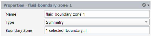
Here, you would typically set the Name, and select the appropriate Boundary Zone for the symmetry fluid boundary. See Symmetry Fluid Boundary Properties for more details.
For additional information, see Symmetry Condition in the Polyflow User's Guide.
In an extrusion problem, where the shape of the extrudate is not known in advance, a free surface is used to represent the outer surface of the extrudate. More generally, a free-surface problem involves a boundary whose position is computed as part of the solution, since it is not known in advance.
When the Type is set to Free surface, use the Fluid Boundary Zone node to access free surface boundary definitions for your simulation (Figure 4.70: Free Surface Fluid Boundary Properties).
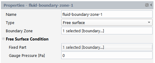
Here, you would typically set the Name, select the appropriate Boundary Zone, and assorted Free Surface Condition properties for the free surface fluid boundary. A free surface usually starts at a point/line where it is fixed. It is even required in steady state calculations. In an extrusion case, the free surface obviously starts at the die exit, so that the intersecting line between the die exit and the free surface is the actual fixed part. A non-zero pressure can also be applied on the free surface. See Free Surface Fluid Boundary Properties for more details.
For additional information, see Free Surfaces and Kinematic Condition in the Polyflow User's Guide.
For extrusion simulations, you can specify two types of extrudate exit conditions. The first condition applies to the edges of the extrudate exit. If all edges are free, the setup corresponds to the calculation of an extrudate shape. If some or all edges are fixed, the setup corresponds to the calculation of die lips shapes (Figure 4.71: Extrudate Exit Fluid Boundary Properties).
In addition to this, a take-up velocity, a take-up force or force density can also be applied on the extrudate exit surface. This is typically the case in fiber spinning where a usually large take-up force or force density is applied, but sometimes also in a simple extrusion situation, where a small force may help stabilizing the process. Note that when die lips shapes are calculated, imposing a take-up force is strongly recommended instead of a take-up velocity.
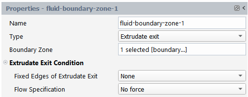
Here, you would typically set the Name, select the appropriate Boundary Zone, and assorted Extrudate Exit properties for the extrudate exit fluid boundary. See Extrudate Exit Fluid Boundary Properties for more details.
For additional information, see Global Force Condition in the Polyflow User's Guide.
A vent boundary condition is typically the boundary condition that can be invoked in a volume of fluid (VOF) simulation where a specific pressure applies at an orifice where the air contained within a mold escapes, until the fluid (polymer) reaches that exit. By extension, the fluid (polymer) can also escape, and this boundary condition can also be used in a classical flow simulation. The gauge pressure is specified, and you may specify whether a zero tangential velocity is imposed.
When the Type is set to Vent, use the Fluid Boundary Zone node to access vent boundary definitions for your simulation (Figure 4.72: Vent Fluid Boundary Properties).
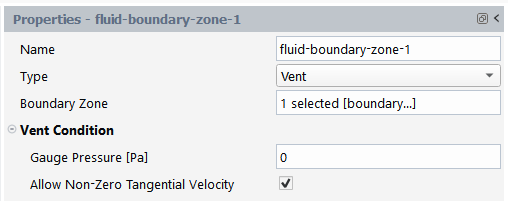
Here, you would typically set the Name, select the appropriate Boundary Zone, and assorted Vent Condition properties for the vent fluid boundary. See Vent Fluid Boundary Properties for more details.
For additional information, see Normal and Tangential Force Condition and Normal Force and Tangential Velocity Condition in the Polyflow User's Guide.
The zero velocity fluid boundary condition simply implies that the normal and tangential velocity components on the boundary are set to zero.
When the Type is set to Zero velocity, use the Fluid Boundary Zone node to access zero velocity fluid boundary definitions for your simulation (Figure 4.73: Zero Velocity Fluid Boundary Properties).
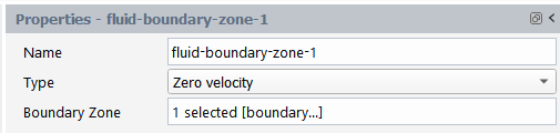
Here, you would typically set the Name, and select the appropriate Boundary Zone for the zero velocity fluid boundary.
The zero force fluid boundary condition simply implies that the normal and tangential force components on the boundary are set to zero.
When the Type is set to Zero force, use the Fluid Boundary Zone node to access zero force fluid boundary definitions for your simulation (Figure 4.74: Zero Force Fluid Boundary Properties).
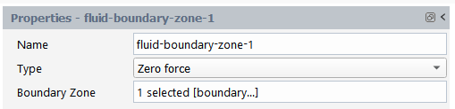
Here, you would typically set the Name, and select the appropriate Boundary Zone for the zero force fluid boundary.
Porous wall conditions are used to model permeable walls. Such walls let some fluid to seep through them and the flow rate will depend on the pressure as in porous medium. Examples of uses for the porous wall condition include screens and filters.
For the porous wall condition (Figure 4.75: Porous Wall Fluid Boundary Properties), a zero tangential velocity component is imposed simultaneously with one of three relationships between the normal force density and the normal velocity. See Porous Wall Condition in the Polyflow User's Guide for details.
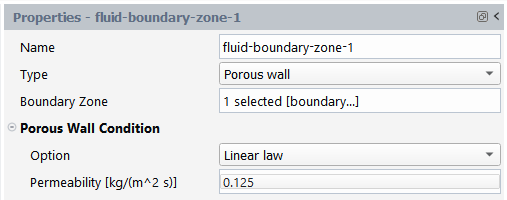
Here, you would typically set the Name, select the appropriate Boundary Zone, and assorted Porous Wall Condition properties for the porous wall fluid boundary.
Porous wall Options include:
Linear: represents a linear relationship between the normal force density and the normal velocity with a constant permeability.
Threshold: represents a porous definition based on two different permeabilities and a critical stress threshold value.
Asymptotic : represents a definition where the growth of the normal force density versus normal velocity is asymptotically bounded to a given value.
See Porous Wall Fluid Boundary Properties for more details.
For additional information, see Porous Wall Condition and Normal Force Calculation in the Polyflow User's Guide.
A force boundary condition should be used when one actually wants to impose a force and not a force density. A force can be typically applied at the exit boundary for an extrusion or fiber spinning simulation, when you want to model a take-up mechanism. Another application is the modelling of a filament stretching experiment. In general, a value is assigned to all three cartesian components of the force. However, only one of them will remain (Figure 4.76: Force Fluid Boundary Properties).
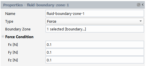
Here, you would typically set the Name, select the appropriate Boundary Zone, and assorted Force Condition properties for the force fluid boundary. See Force Fluid Boundary Properties for more details.
For additional information, see Global Force Condition in the Polyflow User's Guide.
Each of the fluid boundary types include thermal considerations, including an option to select an insulated boundary, to impose a heat flux in different forms, to use an imposed temperature, specify an incoming temperature (for example, restricted to an incoming material) or by using a comma-separated value file. See Thermal Condition Properties for more details.
Each of the fluid boundary types include species considerations which can be defined by selecting the condition for species from the Option drop-down list. The option for species at the fluid boundary will be selected by default, depending on the type of fluid boundary condition. The default option for species for the various fluid boundary types is selected as follows:
Species imposed for Inflow boundary conditions.
Free for Outflow, extrudate exit, and vent boundary conditions.
Symmetry for Symmetry boundary conditions.
Insulated for all other fluid boundary conditions.
When Free, Symmetry, or Insulated are selected, the condition for species at the boundary does not require any user input. However, when Species imposed, Flux, Convection, Flux and convection, or Species profile are selected, additional input is necessary to define the species condition. For more information on defining species conditions see Species Properties as well as Species Condition Properties.
Specify conditions for the solid material(s) at the various boundaries in your simulation (Figure 4.77: Solid Boundary Properties).
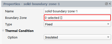
Here you would typically set the Name, select the appropriate Boundary Zone, any Thermal Condition properties if applicable, and for elastic solid zones, specify the solid boundary zone Type. For a solid cell zone that has been defined as elastic, boundary zone types can be defined as Fixed, Free, Symmetry, Normal Displacement, Normal Force Density, Cartesian Displacement, and Force.
For the Normal Displacement and Cartesian Displacement solid boundary zone types, displacement settings for a solid boundary zone can be defined. Similarly, for the Normal Force Density and Force solid boundary zone types, settings can be defined for the force conditions on a solid boundary zone.
The available thermal boundary conditions include an imposed temperature or a temperature profile (using in a CSV file), insulated and symmetry conditions, heat flux, convection, and a combination of both latter ones as well. When appropriate, corresponding parameters are also asked by the program.
For additional information, see Heat Flux Boundary Conditions in the Polyflow User's Guide.
See Solid Boundary Zone Properties for details.
Specify conditions for the porous media at the various boundaries in your simulation (Figure 4.78: Porous Media Boundary Properties).
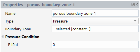
Here, you would typically set the Name, select the appropriate Boundary Zone, the Type, and, if applicable, any Thermal Condition properties for the porous media boundary.
The Type can include: Pressure, Normal velocity, Wall, and Symmetry.
The Pressure boundary condition should be used at inlets and/or outlets; the Normal velocity condition should preferably be used at inlets; the Wall condition should be used along watertight boundaries; and the Symmetry condition should be used along planes of symmetry.
See Porous Boundary Zone Properties for details.
Use the properties of the Contact Boundary Condition (Figure 4.79: Contact Boundary Condition Properties) to describe how and where the fluid and mold come into contact with each other in your simulation.
In blow molding, thermoforming and pressing applications, a fluid, usually polymer or glass, progressively enters into contact with a mold or a plunger or any other solid part involved in the process; this solid part can be either fixed or moving. The occurrence of contact in time and space is a priori unknown. A detection algorithm is invoked, the purpose of which is to detect whether a fluid material point has entered into contact with a solid part or not. As long as a fluid material point is not detected in contact with a solid part, it is free to move in accordance with the forces applied. Once the material point is detected in contact, it acquires the velocity of the solid part. The solver takes care of this treatment, and a penalty mechanism is invoked. Also, when the contact occurs, you may still specify whether the fluid sticks or slips on the contact wall.
Eventually, under some circumstances, contact release is invoked. This is typically the case when a plunger moves back to its former position once it has performed a required action. In the calculation, the contact release indeed occurs when the adhesion force is no longer sufficient for maintaining the contact, in industrial processes, adhesion forces are kept as low as possible to prevent undesirable deformations.
You should specify the surfaces that will enter in contact with each other (fluid surface and solid surface), other quantities must be entered when appropriate.
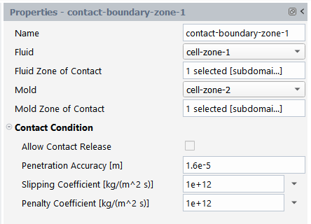
Here, you would typically set the Name, select the appropriate Fluid zone and its Fluid Zone of Contact, the Mold zone, and its Mold Zone of Contact, and any Contact Condition (and, if applicable, any Thermal Condition) properties for the contact boundary.
For additional information, see Working of Contact Detection, Theory and Equations, Penalty Technique for Detecting Contact, and Contact Release in the Polyflow User's Guide.
See Contact Boundary Zone Properties for details.
Specify conditions for a fixed or moving deformable mold at the various boundaries in your simulation.
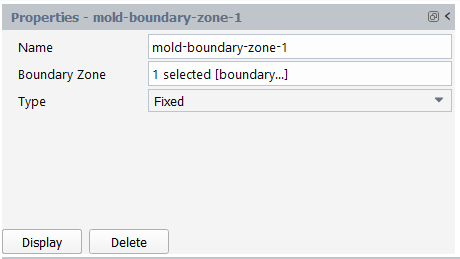
Here, you would typically set the Name, select the appropriate Boundary Zone, and the Type.
The Type can include: Fixed, Free, Symmetry, Normal Displacement, Normal Force Density, and Contact with Fluid.
For a deformable mold simulation to be valid, at least one mold boundary zone with the Type set to Contact with Fluid must be defined. Note that Contact with Fluid is a Post Processor and the simulation of mold deformation is decoupled from the mold-fluid contact simulation.
For the Normal Displacement and Normal Force Density boundary types, conditions can be defined for the displacement and the force density, respectively.
Specify conditions for a restrictor or moving deformable part at the various boundaries in your simulation.
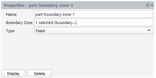
Here, you would typically set the Name, select the appropriate Boundary Zone, and the Type.
The Type can include: Fixed, Free, Symmetry, Normal Displacement, Normal Force Density, and Immersed in Fluid.
For the Normal Displacement and Normal Force Density boundary types, conditions can be defined for the displacement and the force density, respectively.
Use the properties of the Interface Boundary Condition object (Figure 4.82: Interface Boundary Condition Properties) to describe the interaction between adjacent fluids, solids, or porous regions in your simulation.
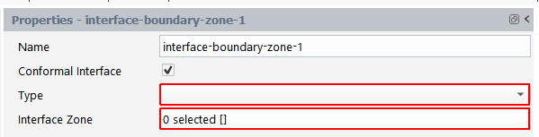
Here, you would typically set the Name, the Type, and select the appropriate Interface Zone for the interface boundary.
The options available for the interface Type are as follows:
For a Conformal Interface:
If two or more fluid cell zones exist, a Fluid-Fluid conformal interface may be defined.
If two or more solid cell zones exist, a Solid-Solid conformal interface may be defined.
If two or more porous media cell zones exist, a Porous-Porous conformal interface may be defined.
If one or more fluid cell zone exists and one or more solid cell zones exist, a Fluid-Solid conformal interface may be defined.
If one or more fluid cell zone exists and one or more porous media cell zones exist, a Fluid-Porous conformal interface may be defined.
If one or more solid cell zone exists and one or more porous media cell zones exist, a Solid-Porous conformal interface may be defined.
For a non-conformal interface (Conformal Interface option disabled):
If two or more fluid cell zones exist, a Fluid-Fluid non-conformal interface may be defined.
For thermal simulations, if two or more inelastic solid cell zones exist, a Solid-Solid non-conformal interface may be defined.
For thermal simulations, if one or more inelastic solid cell zone exists and one or more fluid cell zones exists, a Fluid-Solid non-conformal interface may be defined.
Note that if the interface types described in the above lists are available despite the relevant boundary zone/zones having not been defined, you must change the topology of your mesh within the mesher.
See Interface Boundary Zone Properties for details.
Use the properties of the Fluid-Fluid Interface Boundary Condition object (Figure 4.83: Fluid-Fluid Interface Boundary Condition Properties) to describe the interaction between fluids in your simulation.
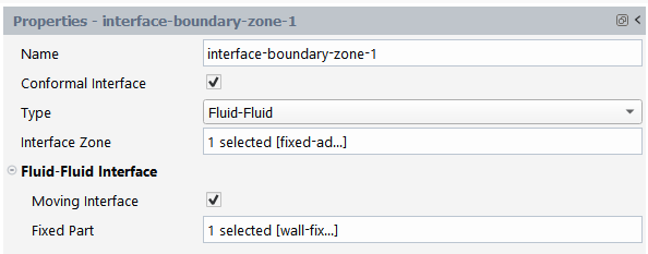
Here, you would typically set the Name, the Type, and select the appropriate Interface Zone for the interface boundary, along with Fluid-Fluid Interface conditions.
Typically, you define a fluid-fluid interface boundary condition between two fluid zones. This interface can be conformal or not. A conformal interface can be a fixed or a moving interface. A fixed interface simulates a gap through which the same fluid can, by default, flow freely between zones. A moving interface simulates a deforming surface separating two fluids.
For more information regarding conformal interfaces, see Kinematic Condition in the Polyflow User's Guide. For more information regarding non-conformal interfaces, see Non-Conformal Boundaries in the Polyflow User's Guide.
See Fluid-Fluid Interface Boundary Zone Properties for details.
Use the properties of the Fluid-Solid Interface Boundary Condition object (Figure 4.84: Fluid-Solid Interface Boundary Condition Properties) to describe the interaction between an adjacent fluid and solid in your simulation.
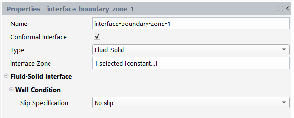
Here, you would typically set the Name, the Type, and select the appropriate Interface Zone for the interface boundary, along with Fluid-Solid Interface (wall) conditions. The settings are similar to the wall fluid boundary condition (see Wall Fluid Boundary for further details).
Typically, you define a fluid-solid interface boundary condition between a fluid and a solid zone. This interface can be conformal or not. When simulating fluid-structure interaction (FSI), a Fluid-Solid interface must be defined for any elastic solid zone that is connected to a fluid region.
For more information regarding non-conformal interfaces, see Non-Conformal Boundaries in the Polyflow User's Guide.
See Fluid-Solid Interface Boundary Zone Properties for details.
Use the properties of the Guiding Device Boundary Condition object (Figure 4.85: Guiding Device Boundary Condition Properties) to describe the interaction between a Guiding Device and a Free surface in your simulation.
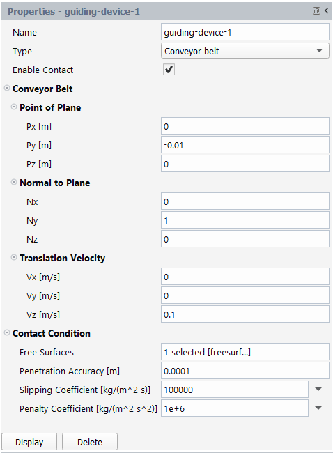
As explained in Understanding Guiding Devices, you can define one or more guiding devices to assist in profile extrusion. A guiding device can be a conveyor belt, a single rotating roller or a roller conveyor made of several rollers. The Guiding Device boundary condition is available for 2D planar and 3D cases after gravity has been specified and at least one free surface has been defined.
Geometric details are discarded when defining the model, and the guiding device is instead defined by its role in the extrusion process. A conveyor belt is represented as a plane and is defined by means of a conveniently selected point and a vector normal to the plane in the outward direction; a translation velocity oriented towards the direction of extrusion is also specified. A rotating roller is represented as a cylinder and is defined by a radius and an oriented axis passing through a given point; a rotation velocity around the axis is also specified. A roller conveyor is a series of identical rollers having the same angular velocity with the same distance between any successive rollers.
The position of the extrudate on the guiding device results from the
equilibrium between gravity in the downward direction and the reaction from the
device acting upwards. For more complex extrusion cases involving guiding
devices, modeling conflicts can occur between the kinematic equation dictating
the extrudate shape and the specified position requirement for the guiding
device. Such conflicts can be resolved by applying an evolution function to
gravity, which will increase the gravitational acceleration as the solution
progresses. For example, defining Gy with the expression -9.81 *
time for a gravitational acceleration of 9.81 in the negative
Y-direction. Additionally, using an expression to define both the slipping
coefficient and the penalty coefficient can improve convergence.
For more information, see Understanding Guiding Devices as well as Guiding Device Boundary Zone Properties.
Depending on the type of simulation you are setting up, it may be necessary to describe a fixed pressure to your enclosed flow domain or a fixed displacement on an elastic solid, deformable mold, or deformable part.
The following sections describe the pressure assignments and displacement assignments in more detail:
Use the properties of the Assign Pressures object (Figure 4.86: Assign Pressure Properties) to describe a fixed pressure to apply to your enclosed flow domain.
Use the New... button to create a new pressure assignment object with its own pressure value and its own location point.
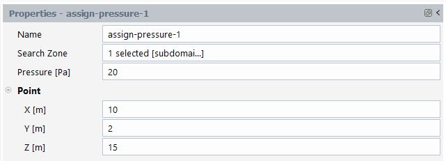
Here, you would typically set the Name, the specific Search Zone or region, the Pressure value for the assignment, along with distinct Point values where the pressure will be assigned.
Note: Pressure assignment is not required when the pressure can be naturally set (such as when a free surface, an inflow/outflow, or an extrudate exit is detected). While the workspace adds a pressure assignment to your simulation automatically if it does not detect an entry, exit, or free surface boundary condition, there are occasions when the pressure assignment is made available but is not necessary (such as when a fluid zone is connected to an adjacent porous or fluid zone).
A pressure assignment is only necessary for flows in a closed domain surrounded only by walls and/or symmetry boundaries, such as flow in a batch mixer, in which case a single pressure assignment is needed at a location that is never overlapped by any moving parts.
See Assign Pressure Properties for details.
Use the properties of the Displacement object (Assign Displacement Properties) to describe a fixed displacement to apply on an elastic solid, deformable part, or deformable mold.
Use the New... button to create a new displacement object with a fixed displacement value at a specified location point.
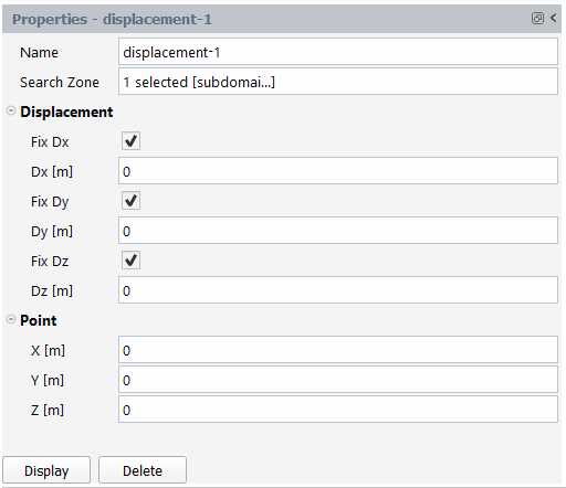
Here, you would typically set the Name, the specific Search Zone or region, the values for the fixed Displacement to be assigned in the x, y, and/or z directions, along with distinct Point values where the displacement will be assigned.
Typically, you would assign a displacement at a point to prevent unwanted rigid translation or rotation that has not been specified through a boundary condition.
See Assign Displacement Properties for details.
Use the properties of the Mesh Deformation object (Figure 4.88: Mesh Deformation Properties) to describe which region deforms during the simulation, and how it deforms.
Note: A mesh deformation entry must be created when there is a free surface or a moving interface whose motion changes the computational domain.
Use the New... button to create a new mesh deformation object. There are different types of mesh deformations: Extrudate, Constant Die Section, Adaptive Die Section, and Lagrangian.
The Extrudate type of deformation is invoked for the deformation of the free jet in extrusion related applications; here you may choose among several deformation methods. Next to the zone, you must also specify its inlet and outlet sections.
The Constant Die Section type of deformation is invoked to deform the die in an extrusion simulation in order to obtain the desired shape of the extrudate while maintaining a constant cross-section in the considered part of the die. This can be combined with the Adaptive Die Section type.
The Adaptive Die Section type of deformation is invoked to deform the outlet cross-section of the considered die part while keeping its original inlet cross-section, the goal being to obtain the desired shape of the extrudate. This can be combined with the Constant Die Section type.
The Lagrangian type of deformation is invoked for transient simulations (blow molding, thermoforming, pressing) where mesh nodes are treated as material points. The zone has to be specified.
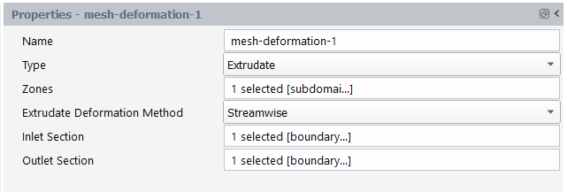
Here, you would typically set the Name, the Type of mesh deformation, select the Zones involved.
For more information, see Remeshing in the Polyflow User's Guide.
See Deformation Properties for details.
In a transient simulation of a shaping process (blow molding, thermoforming, or pressing), the deformations undergone by the fluid are mirrored into the finite element mesh, so that a mesh that was acceptable at the start of the simulation may no longer be adequate later on. Also, for steady and transient cases involving fixed restrictors or moving parts (for example, screws), it is sometimes desirable to locally increase the discretization in order for the fluid to capture the solid part as smoothly as possible. Using the adaptive meshing technique can address these issues.
Depending on the particular context, adaptive meshing features and options are available for the following types of simulations:
Adaptive meshing for blow molding and thermoforming simulations using the shell model, including conditions;
Adaptive meshing for 2D and 3D pressing cases, including conditions and refinement zones;
Adaptive meshing for 2D and 3D simulations involving restrictors or moving parts, including conditions and refinement zones.
In all cases, adaptive meshing requires the selection of general parameters and conditions. In addition, adaptive meshing for 2D and 3D pressing cases allow you to define local refinements.
For blow molding and thermoforming simulations using the shell model, adaptive meshing is based on anticipative element subdivision in order to properly capture the details of the mold shape.
- 4.8.8.1.1. General Properties of Adaptive Meshing for Blow Molding and Thermoforming Simulations Using the Shell Model
- 4.8.8.1.2. Conditions for Adaptive Meshing for Blow Molding and Thermoforming Simulations Using the Shell Model
- 4.8.8.1.3. Contact Conditions Based on Angle and Curvature
- 4.8.8.1.4. Contact Conditions Based on Curvature
- 4.8.8.1.5. Contact Conditions Based on Distance
To display general adaptive meshing properties, in the Outline View, under Setup, select Adaptive Meshing.
![]() Setup → Adaptive
Meshing
Setup → Adaptive
Meshing
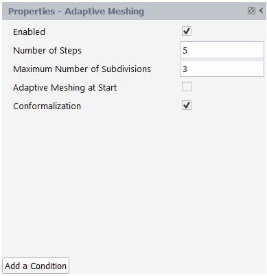
In this case, available properties are displayed in the corresponding Properties page (as shown in Figure 4.89: Properties of Adaptive Meshing for Blow Molding and Thermoforming Simulations Using the Shell Model).
Figure 4.89: Properties of Adaptive Meshing for Blow Molding and Thermoforming Simulations Using the Shell Model
The following properties are available:
- Enabled
Indicate whether or not to use adaptive meshing. By default, adaptive meshing is enabled (the check box is checked). You may disable it by clearing the box; this can be useful for a preliminary trial simulation. When enabled, additional properties are available.
- Number of Steps
Indicate the number of time steps to use for adaptive meshing. A value of 1 indicates that adaptive meshing will take place at each time step. Adaptive meshing is invoked after every sequence of N successful steps, by default N = 5. This is a recommended value as a good compromise between the need of best mesh quality (frequent adaptive meshing) and the necessity of speeding up the calculation (less frequent adaptive meshing). For transient cases, the value should preferably never be less than 4.
- Maximum Number of Subdivisions
Specify the number of times a primitive element. That is, an element of the initial mesh, as created in the mesh generator) can be subdivided recursively.
- Adaptive Meshing at Start
Indicate whether or not to use adaptive meshing at the start of the calculations. That is, for blow molding and thermoforming simulations that involve both contact and adaptive meshing, you can specify that an additional adaptive meshing step is performed before the start of the transient simulation. Adaptive meshing is not enabled at the start of the calculation, by default the check box is cleared. It is assumed that the initial finite element mesh is of acceptable quality, so that an initial adaption step is often not needed. If the initial mesh is of insufficient quality, you may ask for an initial mesh adaption.
- Conformalization
Indicate whether or not to use conformalization on the mesh. For 2D and shell meshes that use the recursive subdivision technique, you can enable conformalization for the mesh. For shells only, conformalization of elements is invoked by default. Adjacent elements are not always subdivided up to the same level, and two smaller elements may be adjacent to a less-subdivided element. A non-conformal situation is created where a middle mesh node may miss a contribution from the adjacent large element. This is internally solved with appropriate constraints. Alternatively, you can invoke mesh conformalization.
To create a new condition for adaptive meshing, select the Add a Condition button at the bottom of the Adaptive Meshing properties panel.
![]() Setup → Adaptive
Meshing
Setup → Adaptive
Meshing
Initially, properties of a condition include:
- Name
Specify a name for the condition, or keep the default value (
condition-1).- Zones
Choose the zone(s) of the fluid region where the specified condition(s) will be applied..
For blow molding and thermoforming, elements in the fluid region are subdivided based on the shape of the mold in front of them; larger elements can be accepted in regions that are in contact with the flat sections of the mold, while smaller elements are needed in regions where the mold is curved. A condition can be defined on the basis of angle and curvature found on the mold, on the basis of curvature only, or on the basis of distance with respect to the mold.
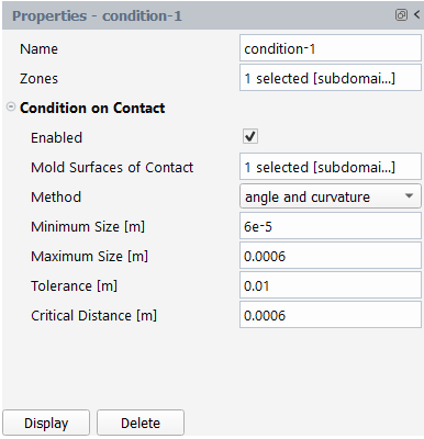
By default, a contact condition is based on angle and curvature. It refines the fluid mesh as it approaches the mold, based on either the angle between neighboring mold elements at a mold node, or on the local curvature of mold elements around a node.
In this case, available properties are displayed in the corresponding Properties page (as shown in Figure 4.90: Contact Condition Properties of Adaptive Meshing Based on Angle and Curvature).
The following properties are available:
- Enabled
Indicate whether or not to consider the condition on contact in order to trigger adaptive meshing. Once a contact condition is enabled (the check box is checked) additional properties are available and you may disable it by clearing the box; note that at least one condition must be enabled.
- Mold Surfaces of Contact
Select the contact zone(s) of the mold to consider for the present contact condition.
- Method
The default method for the condition is based on angle and curvature.
- Minimum Size
Specify the minimum size for newly created elements close to the mold boundary surface. This is the minimum side length of newly created elements, necessary for preventing the creation of a mesh that is too dense. By default, this parameter is assigned a value that is of the order of a tenth of the average edge length in the input mesh.
- Maximum Size
Specify the maximum size for newly created elements far from the mold boundary surface. This is the maximum side length of newly created elements, necessary for preventing the creation of a mesh that is too coarse. By default, this parameter is assigned a value that is of the order of the average edge length in the input mesh.
- Tolerance
For the angle and curvature method, this value defines the tolerance for the contact. This is the maximum distance you would ideally like between any node of the mold and the nearest fluid element. This tolerance is used to locally calculate an ideal fluid element size, in that it could approach the mold within the stated tolerance.
- Critical Distance
For the angle and curvature method, this value has units of length, and is typically 10 percent of the typical size of the segments in the mesh. Note that a larger value results in larger areas of the fluid where the elements are subdivided, which produces higher element counts. On the other hand, if you choose a value that is too small, there may not be sufficient meshing iterations to reduce the elements to an appropriate size. To ensure that is not too small, you must account for the meshing frequency and the velocity of the parison / preform / sheet. The default for this parameter is one percent of the medium diagonal of the axis-aligned minimum box bounding the whole geometry. The critical distance corresponds to an anticipation distance from which mold angles and curvature will have a growing effect on the fluid mesh discretization. It is important to anticipate the contact, for having smaller elements before contact occurrence.
A condition can be defined that is based on only the mold curvature. The condition refines the fluid mesh as the mesh approaches the mold, based on the local curvature of mold elements around a node.
In this case, available properties are displayed in the corresponding Properties page (as shown in Figure 4.91: Contact Condition Properties of Adaptive Meshing Based on Curvature).
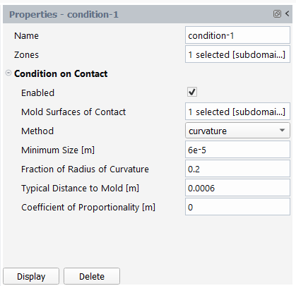
The following properties are available:
- Enabled
Indicate whether or not to consider the condition on contact in order to trigger adaptive meshing. Once a contact condition is enabled (the check box is checked) additional properties are available and you may disable it by clearing the box; note that at least one condition must be enabled.
- Mold Surfaces of Contact
Select the contact zone(s) of the mold to consider for the present contact condition.
- Method
The method for the present condition is based on curvature.
- Minimum Size
Specify the minimum size for newly created elements close to the mold boundary surface. This is the minimum side length of newly created elements, necessary for preventing the creation of a mesh that is too dense. By default, this parameter is assigned a value that is of the order of a tenth of the average edge length in the input mesh.
- Fraction of Radius of Curvature
For the curvature method, this value is dimensionless, and its default value is 0.2. Sufficiently close to the contact mold, element size will be a given fraction of the local radius of curvature, unless it hits the minimum size as lower bound. The selected default value of 0.2 suggests that about 5 fluid elements can be created for matching 1 radian (57 degrees) of a curved mold portion.
- Typical Distance to Mold
For the curvature method, this value has the units of length, and is the typical size of segments of the mesh. This is the distance between a fluid element and the mold below which mesh refinement begins. It is important to anticipate the contact, for having smaller elements before contact occurrence. By default, the value is a fraction of a typical geometric length of the input mesh.
- Coefficient of Proportionality
For the curvature method, this value has units of length. This coefficient may be interpreted as the intended size of the fluid elements when the contact occurs along a flat portion of the mold. For avoiding undesired interferences, either the Fraction of Radius of Curvature or the Coefficient of Proportionality should vanish.
A condition can be defined on the basis of the local distance with respect to the mold only. The condition refines the fluid mesh as the mesh approaches the mold, based on the distance to the mold surface.
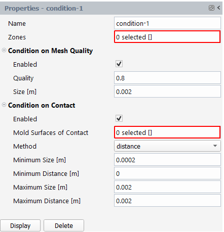
In this case, available properties are displayed in the corresponding Properties page (as shown in Figure 4.92: Contact Condition Properties of Adaptive Meshing Based on Distance).
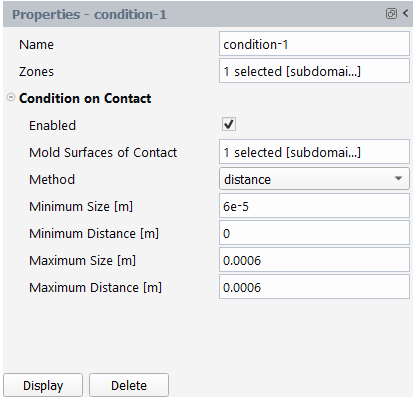
With this method, you only need to specify a simple ramp function that dictates the desired fluid element size versus the distance with respect to the mold. The ramp function specifies a minimum size for fluid elements below a given distance to the mold, a maximum size for fluid elements beyond a given distance to the mold, and a linearly growing size in between.
The following properties are available:
- Enabled
Indicate whether or not to consider the condition on contact in order to trigger adaptive meshing. Once a contact condition is enabled (the check box is checked) additional properties are available and you may disable it by clearing the box; note that at least one condition must be enabled.
- Mold Surfaces of Contact
Select the contact zone(s) of the mold to consider for the present contact condition.
- Method
The method for the present condition is based on distance.
- Minimum Size
Specify the minimum size for newly created elements close to the mold boundary surface. This is the minimum side length of newly created elements, necessary for preventing the creation of a mesh that is too dense. By default, this parameter is assigned a value that is of the order of a tenth of the average edge length in the input mesh.
- Minimum Distance
Specify the minimum distance below which the minimum size is applied. This is the distance between fluid zone and mold below which new fluid elements will be created with the specified minimum size. By default, the minimum distance is set to 0.
- Maximum Size
Specify the maximum size for newly created elements far from the mold boundary surface. This is the maximum side length of newly created elements, necessary for preventing the creation of a mesh that is too coarse. By default, this parameter is assigned a value that is of the order of the average edge length in the input mesh.
- Maximum Distance
Specify the maximum distance beyond which the maximum size is applied. This is the distance between fluid zone and mold beyond which new fluid elements will be created with the specified maximum size. By default, this parameter is assigned a value that is of the order of the average edge length in the input mesh.
For 2D and 3D simulations of pressing cases using volume elements, adaptive meshing is based on mesh triangularization (or tetrahedrization).
In the Outline View, under Setup, select Adaptive Meshing to display general properties.
![]() Setup → Adaptive
Meshing
Setup → Adaptive
Meshing
In this case, available properties are displayed in the corresponding Properties page (as shown in Figure 4.93: Properties of Adaptive Meshing for 2D and 3D Pressing Cases).
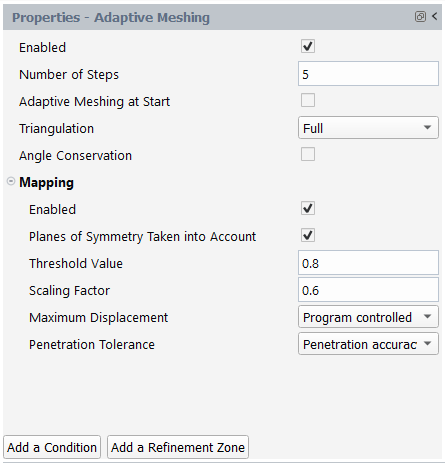
The following properties are available:
- Enabled
Indicate whether or not to use adaptive meshing. By default, adaptive meshing is enabled (the check box is checked). You may disable it by clearing the box; this can be useful for a preliminary trial simulation. When enabled, additional properties are available.
- Number of Steps
Indicate the number of time steps to use for adaptive meshing. A value of 1 indicates that adaptive meshing will take place at each time step. Adaptive meshing is invoked after every sequence of N successful steps, by default N = 5. This is a recommended value as a good compromise between the need of best mesh quality (frequent adaptive meshing) and the necessity of speeding up the calculation (less frequent adaptive meshing). For transient cases, the value should preferably never be less than 4.
- Adaptive Meshing at Start
Indicate whether or not to use adaptive meshing at the start of the calculations. That is, for blow molding and thermoforming simulations that involve both contact and adaptive meshing, you can specify that an additional adaptive meshing step is performed before the start of the transient simulation. Adaptive meshing is not enabled at the start of the calculation, by default the check box is cleared. It is assumed that the initial finite element mesh is of acceptable quality, so that an initial adaption step is often not needed. If the initial mesh is of insufficient quality, you may ask for an initial mesh adaption.
- Triangulation
Indicate whether to use partial or full triangulation for the mesh. If Full triangulation is used, when one element is selected for remeshing, the whole moving domain. That is, the domain for which there are local criteria activated) will be remeshed. With big meshes, the cost of this operation could be too high. Partial triangulation is when one element is selected for remeshing, a zone defined upon the neighbors of this element will be remeshed (and not the entire mesh), and is preferable for large meshes. By default, full triangulation is invoked, and is recommended unless otherwise specified. Full or partial triangulation can be invoked, respectively depending whether the adaptive meshing is applied on the entire fluid mesh or only on portions surrounding elements of bad quality.
- Angle Conservation
Enables angle conservation on the border of the remeshed zone(s). A sequence of adaptive meshing tends to erode sharp borders or edges of a fluid domain. It is especially visible on convex borders. By default, angles are not preserved. Enable this option if you want angles above a given value to be preserved and enter the value. The angle between two adjacent boundary elements is defined as the angle between vectors normal to these elements.
- Angle [deg]
Specify a value for the minimum angle that should be conserved.
Subsequently, settings can be specified for the Mapping, that is, a technique which consists of properly relocating on the contact surface nodes that were already in contact with the mold.
- Enabled
Indicate whether or not to use mapping for the adaptive meshing. A mapping technique is used that projects the nodes along the local normal to the free surface, since the remeshing algorithm used for triangular / tetrahedral element generation builds a new mesh on the basis of the old mesh, rather than the original geometry.
- Planes of Symmetry Taken into Account
Indicate whether or not to account for symmetry planes. A specific mapping treatment is applied in order to preserve planes of symmetry and not geometrically distort them. By default, the option is not enabled and it is recommended unless otherwise specified.
- Threshold Value
This field triggers the mapping of the nodes. The contact algorithm uses internal fields that are named contact_field and are defined on the free surface. This field stores the contact information for each node and initially has a value of either 0 or 1. If a node of the free surface is in contact, the field value is 1, otherwise the value is 0. However, after a remeshing step, the contact_field values must be interpolated onto the newly generated mesh. After this interpolation, the contact_field values are no longer limited to being either 0 or 1, but can be intermediate values. (For example, 0.3). If a node of the free surface has a contact_field value greater than the threshold, the node is assumed to be in contact and will be mapped. The default value of the threshold is 0.8.
- Scaling Factor
This parameter is used to determine if a point on the free surface is in the vicinity of the mold surface. The distance between the free surface point and the mold surface must be less than typical_size*scaling_factor, where typical_size is the maximum size of a face (or a segment in 2D) of the mold surface. By default, the threshold is set to 0.6.
- Maximum Displacement Mode
Allows you to set the method for determining the maximum displacement of surface nodes during the mapping stage of the adaptive meshing as either Program controlled or User Value. It is the upper bound of the displacement applied to nodes that are mapped onto the contact surface. By default, the value is Program Controlled. You can change this and specify a User Value when prompted.
- User Displacement
In order to avoid highly distorted elements in the layer of elements adjacent to the free surface, the displacement of the mapped nodes is limited to this value. A good practice is to define the maximum displacement as 10 to 25 percent of the minimum element size imposed in the adaptive meshing setup. The default value is calculated from the typical mesh size.
- Penetration Tolerance
This parameter is used to provide a tolerance level for the distance between the free surface and the mold surface. If a point on the free surface is located inside the mold at a distance from the mold surface below this tolerance, the point will not be moved; otherwise the position of the point is corrected. Three options are available: a value of max displacement sets the penetration tolerance to be equivalent to the maximum displacement; a value of penetration accuracy sets the penetration tolerance to be equivalent to the minimum of the penetration accuracies; a value of user input allows you to provide your own value for the tolerance.
- User Value
Specify a value for the penetration tolerance, where it is recommended to keep the penetration tolerance to be less than or equal to the penetration accuracy.
To create a new condition for adaptive meshing, select the Add a Condition button at the bottom of the Adaptive Meshing properties panel.
![]() Setup → Adaptive
Meshing
Setup → Adaptive
Meshing
Initially, properties of a condition include:
- Name
Specify a name for the condition, or keep the default value (
condition-1).- Zones
Choose the zone(s) of the fluid region where the condition(s) below will be applied..
For pressing cases, elements in the fluid region are remeshed with a triangulation algorithm. For this, a quality criterion decreasing from 1 (very good) to 0 (very bad) is evaluated. Elements that do not match a specified quality requirement or whose size does not match a given value are ticked for remeshing. In addition to this, specific conditions at the contact boundary can be defined.
Three conditions and their parameters are available where you must enable and define one or both conditions.
A quality criterion decreasing from 1 (very good) down to 0 (very bad) is evaluated, and which incorporates geometric features such as aspect ratio, internal angles, skewness and bending. Elements that do not match a specified quality requirement or do not match an assigned size are ticked for remeshing.
The following properties are available:
- Enabled
Indicate whether or not to consider the condition on the mesh quality in order to trigger adaptive meshing. You may disable it by clearing the box; this can be useful for a preliminary trial simulation.
- Quality
Specify a value for the expected quality of the mesh. A quality criterion decreasing from 1 (very good) down to 0 (very bad) is evaluated, and which incorporates geometric features such as aspect ratio, internal angles, skewness and bending. Fluid elements which do not match the required quality will be adapted. By default, a quality of 0.8 is required.
- Size
Specify a value for the expected element size of the mesh. Fluid elements which do not match the assigned size will be adapted. A default value is evaluated as a fraction of the overall geometric dimension of the mesh. It can be changed.
A condition can be defined on the basis of the mold curvature only, as is the default method. The condition refines the fluid mesh as the mesh approaches the mold, based on the local curvature of mold elements around a node.
In this case, available properties are displayed in the corresponding Properties page (as shown in Figure 4.94: Properties of Pressing-Related Adaptive Meshing Contact Conditions Based on Curvature).
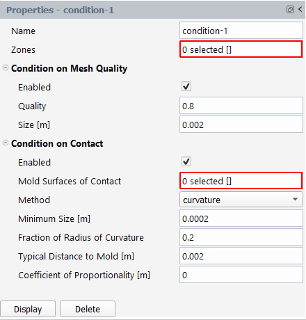
The following properties are available:
- Enabled
Indicate whether or not to consider the condition on contact in order to trigger adaptive meshing. Once a contact condition is enabled (the check box is checked) additional properties are available and you may disable it by clearing the box; note that at least one condition must be enabled.
- Mold Surfaces of Contact
Select the contact zone(s) of the mold to consider for the present contact condition.
- Method
The selected method for the present condition is based on curvature.
- Fraction of Radius of Curvature
For the curvature method, this value is dimensionless, and its default value is 0.2. Sufficiently close to the contact mold, element size will be a given fraction of the local radius of curvature, unless it hits the minimum size as lower bound. The selected default value of 0.2 suggests that about 5 fluid elements can be created for matching 1 radian (57 degrees) of a curved mold portion.
- Minimum Size
Specify the minimum size for newly created elements close to the mold boundary surface. This is the minimum side length of newly created elements, necessary for preventing the creation of a mesh that is too dense. By default, this parameter is assigned a value that is of the order of a tenth of the average edge length in the input mesh.
- Typical Distance to Mold
For the curvature method, this value has the units of length, and is the typical size of segments of the mesh. This is the distance between a fluid element and the mold below which mesh refinement begins. It is important to anticipate the contact, for having smaller elements before contact occurrence. By default, the value is a fraction of a typical geometric length of the input mesh.
- Coefficient of Proportionality
For the curvature method, this value has units of length. This coefficient may be interpreted as the intended size of the fluid elements when the contact occurs along a flat portion of the mold. For avoiding undesired interferences, either the Fraction of Radius of Curvature or the Coefficient of Proportionality should vanish.
A condition can be defined on the basis of the local distance with respect to the mold only. The condition refines the fluid mesh as the mesh approaches the mold, based on the distance to the mold surface.
In this case, available properties are displayed in the corresponding Properties page (as shown in Figure 4.95: Properties of Pressing-Related Adaptive Meshing Contact Conditions Based on Distance).
With this method, you only need to specify a simple ramp function that dictates the desired fluid element size versus the distance with respect to the mold. The ramp function specifies a minimum size for fluid elements below a given distance to the mold, a maximum size for fluid elements beyond a given distance to the mold, and a linearly growing size in between.
The following properties are available:
- Enabled
Indicate whether or not to consider the condition on contact in order to trigger adaptive meshing. Once a contact condition is enabled (the check box is checked) additional properties are available and you may disable it by clearing the box; note that at least one condition must be enabled.
- Mold Surfaces of Contact
Select the contact zone(s) of the mold to consider for the present contact condition.
- Method
The selected method for the present condition is based on distance.
- Minimum Size
Specify the minimum size for newly created elements close to the mold boundary surface. This is the minimum side length of newly created elements, necessary for preventing the creation of a mesh that is too dense. By default, this parameter is assigned a value that is of the order of a tenth of the average edge length in the input mesh.
- Minimum Distance
Specify the minimum distance below which the minimum size is applied. This is the distance between fluid zone and mold below which new fluid elements will be created with the specified minimum size. By default, the minimum distance is set to 0.
- Maximum Size
Specify the maximum size for newly created elements far from the mold boundary surface. This is the maximum side length of newly created elements, necessary for preventing the creation of a mesh that is too coarse. By default, this parameter is assigned a value that is of the order of the average edge length in the input mesh.
- Maximum Distance
Specify the maximum distance beyond which the maximum size is applied. This is the distance between fluid zone and mold beyond which new fluid elements will be created with the specified maximum size. By default, this parameter is assigned a value that is of the order of the average edge length in the input mesh.
To create a new refinement zone for adaptive meshing, select the Add a Refinement Zone button at the bottom of the Adaptive Meshing properties panel.
![]() Setup → Adaptive
Meshing
Setup → Adaptive
Meshing
Initially, properties of a refinement zone include:
- Name
Specify a name for the refinement zone, or keep the default value (
refinement-zone-1).- Type
Specify the method in which you want to define the refinement zone: along boundaries, box, or sphere. For 2D cases, the box and the sphere are respectively reduced to rectangle and circle.
Pressing applications involve large deformations of the mesh; the distortion mainly appears in some localized zones of the mesh. It is therefore interesting to define refinement zones,that is, local regions where the size of the elements must be smaller to catch details of a geometry. Refinement zones can be fixed (in a given region of the space) or moving (defined along a boundary).
You can choose the Type of refinement zone to be a box, defined by two points: a lower-left-front point and a upper-right-back point. Minimum and maximum values of the X, Y and Z-coordinates are required. For 2D cases, Z-coordinates may be set to 0.
In this case, available properties are displayed in the corresponding Properties page (as shown in Figure 4.96: Properties of a Box-Based Refinement Zone).
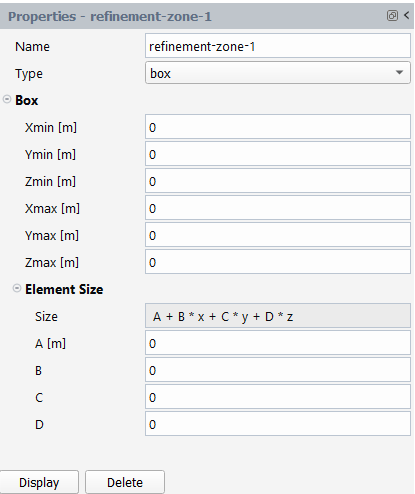
The following properties are available:
- Xmin
Specify a value for the minimum position on the X axis for the refinement zone box (the X-coordinate of the lower-left-front point). The default value is 0.
- Ymin
Specify a value for the minimum position on the Y axis for the refinement zone box (the Y-coordinate of the lower-left-front point). The default value is 0.
- Zmin
Specify a value for the minimum position on the Z axis for the refinement zone box (the Z-coordinate of the lower-left-front point). The default value is 0.
- Xmax
Specify a value for the maximum position on the X axis for the refinement zone box (the X-coordinate of the upper-right-back point). The default value is 0.
- Ymax
Specify a value for the maximum position on the Y axis for the refinement zone box (the Y-coordinate of the upper-right-back point). The default value is 0.
- Zmax
Specify a value for the maximum position on the Z axis for the refinement zone box (the Z-coordinate of the upper-right-back point). The default value is 0.
Inside the defined box, the Element Size distribution is specified as an affine function of the coordinates. The Size is equivalent to A + B * x + C * y + D * z. You should ensure that the size never becomes negative.
- A
Specify the length of the element.
- B
A coefficient for the element size (a coefficient of the affine size function), 0 by default.
- C
A coefficient for the element size (a coefficient of the affine size function), 0 by default.
- D
A coefficient for the element size (a coefficient of the affine size function), 0 by default.
You can choose the Type of refinement zone to be a sphere, defined by the coordinates of its center and a diameter. For 2D cases, the Z-coordinate of the center may be set to 0.
In this case, available properties are displayed in the corresponding Properties page (as shown in Figure 4.97: Properties of a Sphere-Based Refinement Zone).
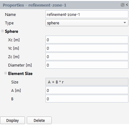
The following properties are available:
- Xc
Specify the X coordinate of the center of the sphere. The default value is 0.
- Yc
Specify the Y coordinate of the center of the sphere. The default value is 0.
- Zc
Specify the Z coordinate of the center of the sphere. The default value is 0.
- Diameter
Specify a value for the sphere diameter. The default value is 0.
Inside the defined sphere, the Element Size distribution is specified as an affine function of the distance with respect to the center. The Size is equivalent to A + B * r. You should ensure that the size never becomes negative.
- A
A constant coefficient for the element size in the spherical refinement zone. The default value is 0.
- B
A coefficient for the affine function for the dependence of the element size with respect to the distance from the center of the spherical refinement zone. The default value is 0.
Having selected the refinement zone Type to be along boundaries, the following properties are available:
- Boundary
Specify a boundary for the refinement zone. For moving zones, specify the free surface on which you want to attach the moving zone.
- Method
Specify the method of refinement along the boundary: distance, or curvature Specifying the size is similar to contacts.
Depending on the selected Method, additional inputs are required.
By default, the refinement method along boundaries is based on the local curvature. It refines the fluid mesh as the local boundary curvature increase (or as the local radius decreases).
In this case, available properties are displayed in the corresponding Properties page (as shown in Figure 4.98: Properties of a Boundary Refinement Zone Based on Curvature).
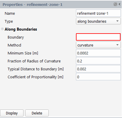
The following properties are available:
- Minimum Size
Specify the minimum size for elements close to the mold boundary. This sets the minimum size for newly created elements close to the selected boundary. By default, this parameter is assigned a value that is of the order of a tenth of the average edge length in the input mesh.
- Fraction of Radius of Curvature
For the curvature method, this value is dimensionless, and its default value is 0.2. Sufficiently close to the selected boundary, element size will be a given fraction of the local radius of curvature, unless it hits the minimum size as lower bound. The selected default value of 0.2 suggests that about 5 fluid elements can be created for matching 1 rad (57°) of a curved boundary portion.
- Typical Distance to Boundary
For the curvature method, this value has the units of length. The typical depth of the zone adjacent to the boundary where elements can be remeshed based on the local curvature. By default, the value is a fraction of a typical geometric length of the input mesh.
- Coefficient of Proportionality
For the curvature method, this value has units of length. This coefficient may be interpreted as the intended size of the fluid elements along a flat portion of the selected boundary. For avoiding undesired interferences, either the Fraction of Radius of Curvature or the Coefficient of Proportionality should vanish.
The refinement method along boundaries can be based on the distance with respect to the selected boundary only. Elements close to the selected boundary will be refined.
In this case, available properties are displayed in the corresponding Properties page (as shown in Figure 4.99: Properties of a Boundary Refinement Zone Based on Distance).
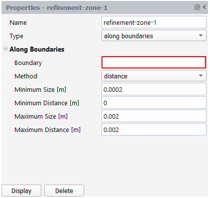
With this method, you only need to specify a simple ramp function that dictates the desired fluid element size versus the distance with respect to the boundary. The ramp function specifies a minimum size for fluid elements below a given distance to the selected boundary, a maximum size for fluid elements beyond a given distance to the selected boundary, and a linearly growing size in between.
The following properties are available:
- Minimum Size
Specify the minimum size for elements close to the mold boundary. This sets the minimum size for newly created elements close to the selected boundary. By default, this parameter is assigned a value that is of the order of a tenth of the average edge length in the input mesh.
- Minimum Distance
Specify the minimum distance below which the minimum size is applied. This is the distance between fluid points and selected boundaries below which new fluid elements will be created with the specified minimum size. By default, the minimum distance is set to 0.
- Maximum Size
Specify the maximum size for elements far from the mold boundary. This sets the maximum size for newly created elements beyond a given distance to the selected boundary. By default, this parameter is assigned a value that is of the order of the average edge length in the input mesh.
- Maximum Distance
Specify the maximum distance beyond which the maximum size is applied. This is the distance between fluid point and selected boundary beyond which new fluid elements will be created with the specified maximum size. By default, this parameter is assigned a value that is of the order of the average edge length in the input mesh.
For steady and transient cases involving restrictors or moving parts, adaptive meshing is based on element subdivision in order to properly capture the details of the restrictors or moving parts. For this, elements are recursively split into sub-elements.
By default, adaptive meshing for cases involving restrictors or moving parts is disabled and must be activated by checking the Enabled checkbox.
In this case, available properties are displayed in the corresponding Properties page (as shown in Figure 4.100: General Properties for Adaptive Meshing Cases Involving Restrictors and Moving Parts).
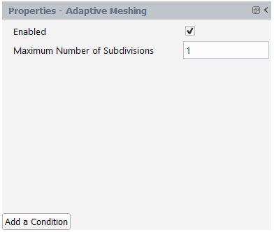
Once enabled, additional properties are available:
- Maximum Number of Subdivisions
Specify the number of times a primitive element. That is, an element of the initial mesh, as created in the mesh generator) can be subdivided recursively.
- Conformalization
Indicate whether or not to use conformalization on the mesh. For 2D and shell meshes that use the recursive subdivision technique, you can enable conformalization for the mesh. For shells only, conformalization of elements is invoked by default. Adjacent elements are not always subdivided up to the same level, and two smaller elements may be adjacent to a less-subdivided element. A non-conformal situation is created where a middle mesh node may miss a contribution from the adjacent large element. This is internally solved with appropriate constraints. Alternatively, you can invoke mesh conformalization.
Now, an overlapping condition can be created and applied to the adaptive meshing scheme.
To create a new condition for adaptive meshing, select the Add a Condition button at the bottom of the Adaptive Meshing properties panel.
![]() Setup → Adaptive
Meshing
Setup → Adaptive
Meshing
Initially, properties of a condition include:
- Name
Specify a name for the condition, or keep the default value (
condition-1).- Zones
Choose the zone(s) of the fluid region where the condition(s) below will be applied..
At least one Condition for Overlapping must be Enabled and defined.
In this case, available properties are displayed in the corresponding Properties page (as shown in Figure 4.101: Properties of an Overlapping Condition for Adaptive Meshing Cases Involving Restrictors and Moving Parts).
Figure 4.101: Properties of an Overlapping Condition for Adaptive Meshing Cases Involving Restrictors and Moving Parts
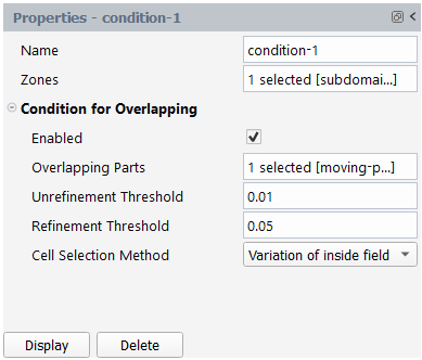
Once enabled, additional options are available:
- Enabled
Indicate whether or not to apply the current condition on overlapping parts for adaptive meshing. When multiple conditions are defined, they may by enabled or disabled at will. Once enabled, additional options are available.
- Overlapping Parts
Select the overlapping part(s) that will be used for mesh adaption in the fluid zone.
- Unrefinement Threshold
Specify the required threshold for local mesh unrefinement. A so-called inside function (or overlapping function) is used to determine whether a fluid element is overlapped by a restrictor or a moving part, or not. It then received the value 1 or 0, respectively. For fluid elements far from the transition stripe, the function exhibits nearly no variation, and they can be selected for unrefinement if the variation is below the threshold value. By default, the threshold value is set to 0.01. The operating mode depends on the cell selection method. For the cell selection method based on inside field variation: when an element of the fluid zone is far enough from the border of the overlapping part. That is, when the corresponding overlapping or inside field exhibits small or no variation), the element can be selected for unrefinement. For the cell selection method based on average inside field values: when an element of the fluid zone is far enough from the overlapping part. That is, when the corresponding overlapping or inside field exhibits small values), the element can be selected for unrefinement.
- Refinement Threshold
Specify the required threshold for local mesh refinement. A so-called inside function (or overlapping function) is used to determine whether a fluid element is overlapped by a restrictor or a moving part, or not. It then received the value 1 or 0, respectively. For fluid elements located near or in the transition stripe, the function exhibits variation, and they can be selected for refinement if the variation is above the threshold value. By default, the threshold value is set to 0.05. The operating mode depends on the cell selection method. For the cell selection method based on inside field variation: when an element of the fluid zone is close enough to the border of the overlapping part. That is, when the corresponding overlapping or inside field exhibits large variation), the element can be selected for refinement. For the cell selection method based on average inside field values: when an element of the fluid zone is close enough to the overlapping part or overlapped. That is, when the corresponding overlapping or inside field exhibits large values), the element can be selected for refinement.
- Cell Selection Method
Specify whether the cell selection method for refinement/unrefinement is based on the variations or on the values of the overlapping or inside field. By default, the selection method for refinement and unrefinement checks the Variation of inside field versus both thresholds. Another method consists of checking the Average of inside field versus both thresholds. The behavior differs since elements overlapped by the solid part will also be refined.