


In an extrusion problem, where the shape of the extrudate is not known in advance, a free surface is used to represent the outer surface of the extrudate. A free-surface problem involves a boundary whose position is computed as part of the solution, since it is not known in advance.
Important: You can also model a free surface on a fixed mesh, using the volume of fluid (VOF) model (see Volume of Fluid (VOF) Model). The VOF model may be more appropriate for flows where the free surface interface is not well defined, such as injection and filling problems.
Free-surface problems have additional degrees of freedom and additional equations, compared with fixed-boundary flow problems. In a fixed-boundary problem, all components of the velocity vector or the surface-force vector can be prescribed. It is also possible to prescribe one velocity component and the other components of the surface-force vector. Prescribing both the normal surface force and the normal velocity, however, would result in an ill-posed problem definition.
For a free-surface problem, the tangential surface force (1 component in 2D, 2 components in 3D), the normal force, and the normal velocity must all be prescribed. Two requirements must be satisfied: the dynamic condition and the kinematic condition.
In the absence of surface tension in a steady-state flow, the position of the free surface must be prescribed upstream of the free surface.
The normal force  must be equal to zero, or more generally, be prescribed a
given value
must be equal to zero, or more generally, be prescribed a
given value  :
:
 | (15–1) |
where  is nonzero when an external force is applied on the free
surface. For example, when an internal pressure is applied in a blow-molding
application,
is nonzero when an external force is applied on the free
surface. For example, when an internal pressure is applied in a blow-molding
application,  is not zero. This condition (Equation 15–1) is referred to as the dynamic condition. For free surfaces, this condition
is prescribed as a Neumann boundary condition for the momentum equation.
is not zero. This condition (Equation 15–1) is referred to as the dynamic condition. For free surfaces, this condition
is prescribed as a Neumann boundary condition for the momentum equation.
For steady-state flows, the normal velocity must be equal to zero:
 | (15–2) |
where  is the velocity vector and
  is the normal vector to the free surface. Equation 15–2 states that no mass crosses the free surface, in the case of a steady-state
problem. This condition is referred to as the kinematic condition.
is the normal vector to the free surface. Equation 15–2 states that no mass crosses the free surface, in the case of a steady-state
problem. This condition is referred to as the kinematic condition.
For time-dependent problems, the kinematic condition becomes
 | (15–3) |
where  is the position of a node on the free surface.
Equation 15–3 states that a time-dependent free surface must follow trajectories in the normal direction, while the tangential displacement is not restricted. When Equation 15–3 is implemented in a finite-element code, it is correct to describe it as the requirement that nodes located on a free surface are Lagrangian in the normal direction.
In order to be well-posed, a free-surface problem requires a new scalar degree
of freedom, called the geometrical degree of freedom. The geometrical degree of
freedom is denoted by  , which describes the amplitude of the displacement of boundary
nodes in the normal direction. This mixture of a Lagrangian description in the
normal direction and an Eulerian description elsewhere is sometimes referred to
as an Arbitrary Lagrangian-Eulerian (ALE) formulation.
, which describes the amplitude of the displacement of boundary
nodes in the normal direction. This mixture of a Lagrangian description in the
normal direction and an Eulerian description elsewhere is sometimes referred to
as an Arbitrary Lagrangian-Eulerian (ALE) formulation.
It can be shown that it is possible to satisfy Equation 15–1 and Equation 15–2 (for steady-state problems), or Equation 15–1 and Equation 15–3 (for time-dependent problems) provided that the direction in which boundary nodes are allowed to move never becomes tangent to the moving surface, which is evaluated as a function of the solution itself. If this condition is violated, Ansys Polyflow will print an error message signaling a vanishing pivot for the geometrical degree of freedom. As the violation is approached (that is, as the direction of the motion approaches the local tangential direction), the calculation may also diverge.
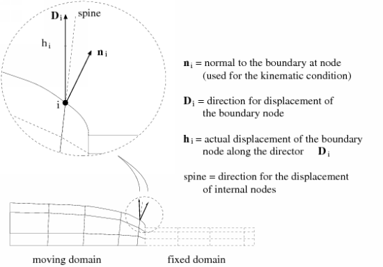
In Ansys Polyflow, the direction of displacement for the boundary nodes
( ) is prescribed in advance, and the amplitude of the
displacement is the geometrical degree of freedom (
) is prescribed in advance, and the amplitude of the
displacement is the geometrical degree of freedom ( ), except for the line kinematic condition.
  is referred to as the director. Although the director
 is a given and not a variable of the problem, each node has
its own director, and Ansys Polyflow provides automatic tools for evaluating
default directors. Unless otherwise specified, directors are the local normals
to the initial mesh. Figure 15.1: Definition of Displacement, Spine, and Normal Directions
describes the relationship between the
is a given and not a variable of the problem, each node has
its own director, and Ansys Polyflow provides automatic tools for evaluating
default directors. Unless otherwise specified, directors are the local normals
to the initial mesh. Figure 15.1: Definition of Displacement, Spine, and Normal Directions
describes the relationship between the  and
and  directions. Note that
  is different from the direction of a spine used for remeshing
(see Remeshing).
is different from the direction of a spine used for remeshing
(see Remeshing).
See Directors for details about directors.