


The Solution section of the Outline View and the Ribbon allow you access to common solution-specific controls, such as:
It is necessary to initialize the temperature wherever it is defined. Temperature
fields can be initialized either by specifying the components of the temperature
initialization equation or by importing a CSV file of a temperature profile. The
temperature initialization equation is T = A * ( 1 + B * x + C * y
) for 2D meshes, and T = A * ( 1 + B * x + C * y + D * Z
) for 2D shell/3D meshes. For steady or continuation calculation types,
temperature initialization should be as close as possible to the targeted solution
to facilitate convergence.
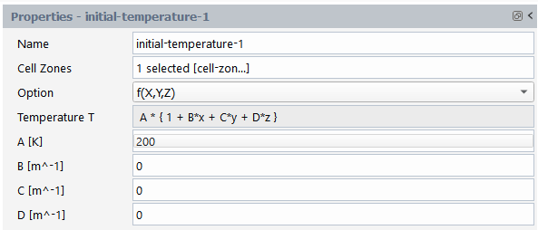
See Temperature Initialization Properties for details.
It is necessary to initialize species transport equations wherever they are
defined. Species transport can be initialized either by specifying the components of
the species initialization equation or by importing a CSV file of a species profile.
The species initialization equation is S = A * ( 1 + B * x + C * y
) for 2D meshes and S = A * ( 1 + B * x + C * y + D * Z
) for 3D meshes. For steady or continuation calculation types, species
initialization should be as close as possible to the targeted solution to facilitate
convergence.
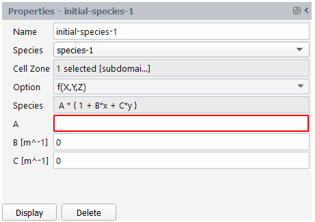
See Species Properties for details.
Use the Probes task to create discretely located points in your domain to monitor your simulation.
Use the New... button to create a new point object (Figure 4.104: Properties of Probe). Once you specify the x, y, and Z coordinates, you can indicate whether the point will a Moving node (the field values will be extracted at a material point that can move with time), or a Fixed geometric location (field values will be extracted at the provided coordinates whatever the motion of the material).
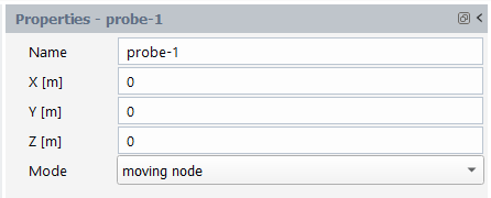
Here, you would typically set the Name, and the X, Y, and Z coordinates of the solution probe.
See Probe Properties for details.
Use the Derived Quantities task to determine which of the available derived quantities you want to create an output field for within your simulation.
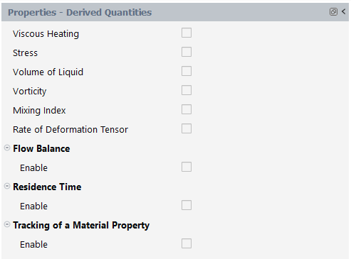
The choices for Derived Quantities can include:
Table 4.10: Available Derived Quantities
| Quantity | Availability | Default Setting | |
|---|---|---|---|
| Shear Rate - local shear rate in the flow domain. |
Available if the domain is not shell and if there is at least one fluid cell zone |
Enabled. | |
| Viscosity - local viscosity in the flow domain. |
Available if the domain is not a shell and if there is at least one fluid cell zone with a Generalized Newtonian fluid model or with a Simplified Viscoelastic model. |
Enabled. | |
| Viscous Heating - local viscous heating in the flow domain, friction heating along walls (if partial slippage is defined), dissipated power. |
Available if the domain is not a shell and if there is at least one fluid cell zone with a Generalized Newtonian fluid model or with a Simplified Viscoelastic model. |
Enabled by default if the simulation is thermal, otherwise it is disabled. | |
| Stress - local stress in the flow domain, includes the evaluation of eigenvalues, N1 and vTv. |
Available if the domain is not shell and if there is at least one fluid cell zone. |
Disabled. | |
| Volume of Liquid - volume of the flow domain. |
Available if the domain is not shell and if there is at least one fluid cell zone. |
Enabled and read-only if VOF simulation, otherwise disabled. | |
| Tracking of Material Points - tracking initial position of fluid points in transient simulations. |
Available if the domain is not shell, if the simulation is transient and if there is at least one fluid cell zone. |
Disabled. | |
| Vorticity - local vorticity tensor |
Available if the domain is not a shell and if there is at least one fluid cell zone. |
Disabled. | |
| Mixing Index - local mixing index |
Available if the domain is not a shell and if there is at least one fluid cell zone. |
Disabled. | |
| Rate of Deformation Tensor - local tensor D |
Available if the domain is not shell and if there is at least one fluid cell zone. |
Disabled. | |
| Force - resulting force on each fluid boundary condition will be written in the transcript. |
Available if the domain is not shell and if there is at least one fluid cell zone. |
Disabled. | |
| Flow Rate - resulting volumetric flow rate on each fluid boundary condition. |
Available if the domain is not a shell, if there is at least one fluid cell zone. |
Enabled. | |
| Heat Flux - resulting heat flux on each fluid, solid, porous boundary condition will be written in the transcript file. |
Available if the domain is not shell, the simulation is thermal and if there is at least one cell zone of type fluid, solid or porous. |
Enabled. | |
| Flow Balance - quantification of die balancing. |
Available if the flow rate postprocessor is available and enabled. |
Disabled. | |
| Convective Heat - transported heat on each fluid boundary condition. |
Available if the domain is not a shell, the simulation is thermal and if there is at least one fluid cell zone. |
Enabled. | |
| Residence Time - residence time of fluid points entering the fluid domain. |
Available if the domain is not shell and if there is at least one inlet fluid boundary condition. You must specify the fluid boundaries where it will be initialized and provide the initial value. |
Disabled. | |
| Tracking of a Material Property - tracking a property of fluid points entering the fluid domain. |
Available if the domain is not a shell, if the simulation is transient and if there is at least one fluid cell zone |
Disabled. | |
| Extension - evaluation of the extension components for blow molding and thermoforming simulations. | Area Ratio: for each face of the fluid domain, ratio of the face surface to the initial face surface | Available if the domain is a shell. |
Enabled. |
| Track Vectors: local deformations of specified vectors |
Disabled. | ||
| Self Contact - contact detection of the polymer sheet with itself. |
Available if the domain is a shell. |
Disabled. | |
| Estimated Thickness - evaluation of the thickness of a product. |
Available if the domain is not a shell and not a film, and if the simulation is transient with no restrictors or moving parts. |
Disabled. | |
Note: Depending on the type of simulation (blow molding, extrusion, etc.), relevant quantities are already enabled, and you can disable them if desired. For instance, Shear Rate in transient simulations may be too computationally expensive, and Flow Balance, Residence Time, and Tracking of Material Points require additional information.
Once selected, when a solution is generated, these quantities will be available for postprocessing (see Postprocessing Results).
Note: Some derived quantities/fields are created automatically, such as those for mesh quality whenever you have a deforming mesh. See Analysing Mesh Quality for more information.
The workspace can calculate the local shear rate ( ) on the part of the domain where the velocity field has been
calculated. The shear rate is given by
) on the part of the domain where the velocity field has been
calculated. The shear rate is given by
 | (4–9) |
Properties include:
- Shear Rate
Enable this option to create an output field to evaluate the shear rate.
For generalized Newtonian fluids and simplified viscoelastic fluids, the workspace can calculate the local value of the viscosity, which can depend on the shear rate and/or the temperature. The viscosity will appear as a scalar field while postprocessing.
Properties include:
- Viscosity
Enable this option to create an output field to evaluate the viscosity.
For generalized Newtonian models and simplified viscoelastic fluids, the workspace can calculate the heat generation per unit time and per unit volume (or per unit area for a 2D planar case) that is generated under the given flow conditions. The heat generation originates from the work of internal forces. In addition to the viscous and wall friction heating, the workspace evaluates the dissipated power, which is the integral of the viscous and wall friction heating over the flow domain. When wall slippage is defined, the calculation of the dissipated power also considers the contribution originating from the slipping force, and results are provided for the volume dissipated power and the heat generated from slipping.
It is not necessary to solve a nonisothermal problem in order to compute the viscous and wall friction heating. The workspace can calculate the viscous dissipation that occurs without actually solving the energy equation. Also, the workspace can calculate the viscous and wall friction heating even if it has been neglected in the main nonisothermal flow problem.
Properties include:
- Viscous Heating
Enable this option to create an output field containing the local intensity of viscous dissipation (heat generation by friction of fluid layers and slipping)
For generalized Newtonian model, the workspace can calculate the extra-stress
tensor  on the part of the domain where the velocity field has been
calculated. Three components of the inelastic stress tensor will be calculated
for 2D planar cases, four components for 2D axisymmetric cases, and six
components for all other cases.
on the part of the domain where the velocity field has been
calculated. Three components of the inelastic stress tensor will be calculated
for 2D planar cases, four components for 2D axisymmetric cases, and six
components for all other cases.
For differential or simplified flow problems, the workspace can calculate the total extra-stress tensor in the domain. The total extra-stress tensor is the sum of the viscous (or the (generalized) Newtonian) components and the viscoelastic components. If more than one relaxation time has been defined, the viscoelastic component is the sum of the viscoelastic components for all modes.
Properties include:
- Stress
Enable this option to create an output field containing the stress tensor (stresses in the fluid due to fluid deformation)
With this postprocessor, you can evaluate the volume of the flow domain. If the flow domain contains overlapping internal restrictor or moving parts, the calculation of the volume will remove the part of the flow domain overlapped by these parts, in order to provide the actual volume occupied by the fluid.
Properties include:
- Volume of Liquid
Enable this option to create an output field to evaluate the volume of the flow domain.
In time-dependent calculations, it is sometimes necessary to calculate the trajectory of material points, the workspace is not a Lagrangian code (that is, it does not use a description and formulation following the particles), and nodes do not correspond, in general, to material particles. Therefore, a postprocessor is provided to track these material points. Typically this is useful in blow molding simulations, when remeshing is not of the Lagrangian type, although it can be very useful in many other situations also.
- Tracking of Material Points
Enable this option to create an output field for tracking material particles.
This is available if the domain is not a shell and if there is at least one inlet fluid boundary condition. In addition, you should specify the fluid boundaries where it will be initialized and specify the initial value.
Properties include:
- Enable
Activates the tracking of material particles.
A material particle’s initial position is tracked according to
 | (4–10) |
where  is the initial position of the material particle (that is,
the original position before deformation occurs). When the material points
postprocessor is used, the workspace will keep track of the initial position
of each material point, as well as the final position of that same material
point. This allows you, for example, to determine the source on the parison
of a flaw that occurs at a particular location on the final product. This
post-processor is valid for transient cases defined on a material volume,
i.e. without entry and exit.
is the initial position of the material particle (that is,
the original position before deformation occurs). When the material points
postprocessor is used, the workspace will keep track of the initial position
of each material point, as well as the final position of that same material
point. This allows you, for example, to determine the source on the parison
of a flaw that occurs at a particular location on the final product. This
post-processor is valid for transient cases defined on a material volume,
i.e. without entry and exit.
 | (4–11) |
The mixing index  is defined as
where  is the equivalent shear rate defined as
 | (4–12) |
In a purely rotational flow, the mixing index is zero. The mixing index is not defined everywhere in the flow problem; singular values arise in regions where the denominator is zero (for example, along the axis of symmetry of a Poiseuille flow).
and  is the magnitude of the vorticity vector. For a shear flow,
the mixing index is equal to 0.5, whereas its value is 1 in a purely
elongational flow.
is the magnitude of the vorticity vector. For a shear flow,
the mixing index is equal to 0.5, whereas its value is 1 in a purely
elongational flow.
The mixing index will appear as a scalar during postprocessing.
Properties include:
- Mixing Index
Enable this option to create an output field to evaluate the mixing index lambda (λ)
The workspace can calculate the vorticity vector  for the flow. Vorticity is a measure of the rotation of a
fluid element as it moves in the flow field, and is defined as the curl of the
velocity vector:
for the flow. Vorticity is a measure of the rotation of a
fluid element as it moves in the flow field, and is defined as the curl of the
velocity vector:
 | (4–13) |
This quantity is a vector representation of twice the antisymmetric part
 of the velocity gradient tensor given by
 | (4–14) |
For 3D flows, the vorticity vector  is given in component form by
 | (4–15) |
For 2D planar and axisymmetric flows, the vorticity has one non-zero component only, and it is displayed as a signed scalar quantity. For 2D 1/2 flows, the magnitude of the vorticity vector is displayed, while it will appear as a vector while postprocessing for 3D flows.
Properties include:
- Vorticity
Enable this option to create an output field to evaluate the vorticity.
The workspace can calculate the rate-of-deformation tensor  on the part of the domain where the velocity field has been
computed. Three components of the rate-of-deformation tensor will be calculated
for 2D planar cases, four components for 2D axisymmetric cases, and six
components for all other cases.
on the part of the domain where the velocity field has been
computed. Three components of the rate-of-deformation tensor will be calculated
for 2D planar cases, four components for 2D axisymmetric cases, and six
components for all other cases.
Furthermore, the components are based on the selected reference frame (Cartesian for 2D planar and 3D cases, cylindrical for axisymmetric cases). In many cases, the calculation of the local shear rate (see Shear Rate) is preferred if only a (generalized) scalar kinematics quantity is needed.
Properties include:
- Rate of Deformation Tensor
Activates the calculation of the rate-of-deformation tensor D in the flow domain.
The workspace can calculate the resulting forces applied from the fluid to the several boundaries. The result is evaluated independently for each boundary and is printed in the transcript. Enabling this option allows you to know the corresponding force needed for satisfying the imposed flow boundary condition.
Properties include:
- Force
Enable this option to create an output field to evaluate the force.
The workflow automatically integrates the total volumetric flow rate along all
boundary sets. Results are displayed as numerical values in the transcript
(search for the word Flow rates to find them).
Properties include:
- Flow Rate
Enable this option to create an output field to evaluate the flow rate.
For thermal cases, the workspace can calculate the resulting heat fluxes which leaves the domain through the several boundaries. The result is evaluated independently for each boundary and is printed in the transcript. Enabling this option allows you to know the corresponding heat flux needed for satisfying the imposed temperature boundary condition.
Properties include:
- Heat Flux
Enable this option to create an output field to evaluate the heat flux.
Die balancing is a major challenge for the die designer. To help address this challenge, the workspace can compute a measure of the die balancing based on the deviation of the normal velocity with respect to the average velocity along the die exit:
 | (4–16) |
where  is the velocity,
  is the flow rate across the boundary set,
  is the surface of the boundary set, and
  is the outward normal along the boundary set.
A perfectly balanced die with a uniform velocity at the exit leads to a
measure of the die balancing equal to zero. This measure is not absolute; you
have to compare the die balancing measure for different die geometries to
determine which is the best one (that is, the one with the smallest value for
the die balancing measure). Results are displayed as numerical values in the
workspace transcript (search for the words Flow balance
to find them).
Properties include:
- Enable
Activates the evaluation of the uniformity of the velocity field at specified boundary(ies)
- Useful Borders
Select the boundary(ies) where the flow balance will be evaluated.
This postprocessor is available for boundaries of fluid zones in thermal simulations. Only boundaries with non-zero normal velocity should be considered. Indeed, along walls or plane of symmetries, the convected heat should be zero.
The convected heat postprocessor computes the integral along selected
boundaries of  , where
  is the temperature.
- Convected Heat
Activates the evaluation of the convected heat field. Convected heat is evaluated automatically for each fluid boundary condition.
The workspace can calculate the residence time distribution in the part of the domain where a velocity field has been calculated. The residence time distribution can be calculated in 2D and 3D calculations in steady-state and time-dependent modes. This postprocessor differs from individual time integration along a trajectory, where the result is obtained for a single material point only. With this postprocessor, a residence time distribution value is obtained over the whole domain.
- Enable
Activates the evaluation of the residence time in the flow domain.
- Inlet Boundary
Select the boundary(ies) where the residence time is imposed.
- Law
Select the law for imposing the residence time such as Constant or Polynomial.
- A
Specify a value for the constant coefficient of the residence time function at the inlet boundary.
- B
Specify a value for the X coefficient of the polynomial function for the residence time function at the inlet boundary.
- C
Specify a value for the Y coefficient of the polynomial function for the residence time function at the inlet boundary.
- D
Specify a value for the Z coefficient of the polynomial function for the residence time function at the inlet boundary.
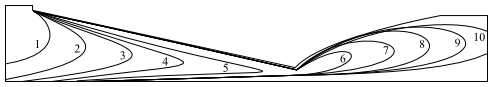
Consider a simple steady-state free surface flow, where the flow enters from the upper left part of the domain. Assuming that the residence time distribution is zero in the entry section, the workspace will calculate the residence time distribution in the domain. An example of contour lines of the residence time distribution is shown in Figure 4.106: Contour: Residence Time Distribution for a Steady-State Free Surface Problem.
The workspace computes the residence time distribution using the equation
 | (4–17) |
where  at time
  , and the boundary conditions along the entry sections are
taken into account.
, and the boundary conditions along the entry sections are
taken into account.  is the residence time, and
  is the material derivative of the residence time.
Equation 4–17
states that the residence time increases as the absolute time
 for particles along their path increases. It is a
hyperbolic equation, and it requires boundary conditions (as well as initial
conditions for time-dependent problems). The value of the residence time
must be set along all entry sections.
for particles along their path increases. It is a
hyperbolic equation, and it requires boundary conditions (as well as initial
conditions for time-dependent problems). The value of the residence time
must be set along all entry sections.
Usually you will set a value of zero. On all sections on which an inflow boundary condition has been applied for the momentum equation, the residence time is set to zero by default. You can add boundary conditions on entry sections where a different type of condition has been selected.
For time-dependent calculations, the workspace imposes
 as an initial condition. In this case, the time-dependent
problem is well-posed provided that
as an initial condition. In this case, the time-dependent
problem is well-posed provided that  has been imposed on all entry sections. For steady-state
problems, Equation 4–17 does not define a well-posed problem in recirculating
zones (vortices) and along walls where
has been imposed on all entry sections. For steady-state
problems, Equation 4–17 does not define a well-posed problem in recirculating
zones (vortices) and along walls where  .
.
This is not usually important, since the residence time distribution is meaningless in these regions, and you can easily exclude these corresponding contour lines from the display in your graphical postprocessing program.
Another possibility for calculating the residence time distribution in the presence of steady-state vortices is to define a time-dependent problem that uses a steady-state velocity field that has already been calculated.
For flow problems, you can track particles by assigning a value of a material
property (a conventional scalar field named  for "color") in the flow domain and integrating the pure
advection of this property in the flow domain:
for "color") in the flow domain and integrating the pure
advection of this property in the flow domain:
 | (4–18) |
Equation 4–18 is subject to inlet boundary conditions that can be defined separately on
each inlet section. This postprocessor is typically used to calculate the
transport of the property in the flow. Each separate entry has a different color
represented by a separate value of the  property along the inlet. The flow transports the property and
you can locate the color at each position in the flow domain.
property along the inlet. The flow transports the property and
you can locate the color at each position in the flow domain.
The continuous interpolation used in the numerical scheme will produce some interpolation error, so intermediate values will also be displayed in the flow domain. However, provided you select distinct values of the property along inlets (such as 1 and 10, for example), you can easily identify regions of the flow during postprocessing.
Properties include:
- Inlet Boundary
Select the boundary(ies) where the material property is imposed.
- Law
Select the law for imposing the material property such as Constant or Polynomial.
- A
Specify a value for the constant coefficient of the material property function at the inlet boundary.
- B
Specify a value for the X coefficient of the polynomial function for the material property function at the inlet boundary.
- C
Specify a value for the Y coefficient of the polynomial function for the material property function at the inlet boundary.
- D
Specify a value for the Z coefficient of the polynomial function for the material property function at the inlet boundary.
Evaluation of the extension components is available for blow molding and thermoforming simulations. This is available if the domain is a shell. Two kinds of extensions can be evaluated:
- Area Stretch Ratio
Indicate whether or not to evaluate the distribution of area stretch ratio undergone by the fluid zone, that is, the ratio of local area after deformation to initial area.
- Track Vectors
Activates the evaluation of the deformations of specified vectors in the flow domain.
You must specify the Initial Orientations of the vectors: initially parallel to the direction D, initially perpendicular to the direction D, initially radial from point P, initially circumferential around point P (where more than one can be selected at once). You must then specify the coordinates of the reference point P and orientation of the vector D.
You must specify the coordinates of the reference point P.
- Px
Specify the x-coordinate of the reference point P.
- Py
Specify the y-coordinate of the reference point P.
- Pz
Specify the z-coordinate of the reference point P.
For blow molding and thermoforming processes in shell models, there are times when self-contacts such as folds or knit-lines can occur in the blown part. In such cases, the self-contact postprocessor can simply detect self-contact of the parison.
- Enable
Activates the detection of folds or knit-lines that can occur in a blown/thermoformed part.
- Action
Select the action to be taken when self-contact is detected such as No action, Warning or Stop. No action simply allows to postprocess the self-contact field. Warning generates a message in the transcript. Stop halts the calculation.
In 2D as well as in 3D simulations of blow molding and pressing, you can compute the thickness of the final object (as well as during shaping). In industrial processing, the thickness has to be understood as the distance between two arbitrary surfaces; it is therefore subjected to an appropriate definition. Also, from the point of view of modeling, it would require the identification of preferably distinct topological entities; however this cannot always be achieved. A technique has been implemented, which matches a reasonable industrial definition as much as possible: at a given point, it basically consists of evaluating the distance with respect to the closest opposite surface. A topological object has to be constructed for the thickness evaluation, and a few parameters for geometric tolerances have to be given. In 3D, the thickness is evaluated on the selected boundary; planes of symmetry can be discarded from the domain of evaluation. Note that in 2D, a similar scenario applies; however, since the display of a quantity along a line is not easy, the evaluation is expanded onto the domain via a Laplace equation.
Typically, the thickness at the end of the process is of interest. Hence, it is not necessary to perform a thickness evaluation at each time step. Also, since the thickness at a point is evaluated as a distance measured along a line perpendicular to the surface at this point, it is preferable to bound its value.
- Zones
Select the zone(s) where the derived quantity must be calculated.
- Useful Borders
Specify the border that is used as the basis for the evaluation of the thickness; it may consist of one or several boundaries, but typically symmetry planes and lines are not considered.
- Activation Time
Specify a value for the activation time. The thickness evaluation will be performed only when the simulation time is greater than or equal to the activation time.
- Tolerance
Specify a value for the geometric tolerance. The thickness at a point is evaluated as a distance between the point and the opposite surface, measured along a line perpendicular to the surface at this point. The algorithm involves a search of geometric intersection (between the perpendicular line and boundary elements). A geometric tolerance is needed in order to compensate for round-off errors.
The Fluent Materials Processing workspace automatically creates mesh quality fields when the mesh deforms during the calculation. These fields allow you to analyze the mesh and identify distorted elements.
The mesh quality fields are:
MAX_ANGLE: the widest angle found between two successive edges of (a face of) an element
MIN_ANGLE: the narrowest angle found between two successive edges of (a face of) an element
MAX_ASPECT_RATIO: the ratio of the lengths of the longest edge to that of the shortest edge of an element
MAX_BEND: evaluated as one minus the cross product between unit normal directions defined at two opposite vertices of a quadrilateral.
MAX_SKEW: see Element Distortion Check for more information.
The best way to evaluate mesh quality in the Fluent Materials Processing workspace is to create isosurfaces of the mesh quality fields to locate distorted elements. The minimum and maximum values displayed in the iso-surface property panel also allow you to gauge mesh distortion.
An interior angle is defined as the angle between two adjacent edges at a vertex. For example, the interior angles of a square are of 90 degrees, while the angles of an equilateral triangle are of 60 degrees. By default, the minimum and maximum angles are set to 5 and 170 degrees, respectively.
The aspect ratio of an element is defined as the ratio of the lengths of the longest edge to that of the shortest edge. By default, a maximum aspect ratio of 10 is set.
The bend is evaluated based on the cross product between unit normal
directions  and
and  defined at two opposite vertices of a quadrilateral
defined in the plane or in the space. More precisely, it is defined as
defined at two opposite vertices of a quadrilateral
defined in the plane or in the space. More precisely, it is defined as
 . Obviously for a triangular face, the bend is always zero
and consequently a tetrahedron is never bent. A regular quadrilateral face
has also a zero bend; however, the bend of a quadrilateral in the space may
equal 1 or 2 when an edge is rotated by 90 or 180 degrees out of the plane
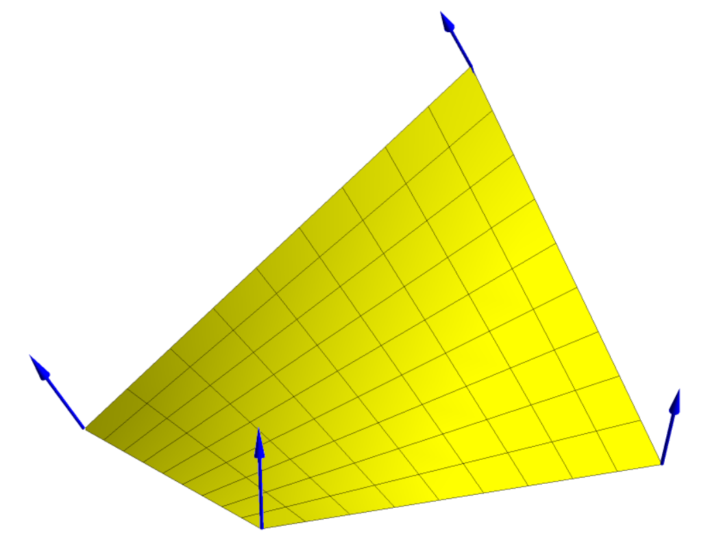
of the quadrilateral, respectively. The element displayed in Figure 4.107: Bent Quadrilateral and Unit Normal Directions at Vertices is obtained by lifting one vertex
of a square element in the upward direction over a distance that corresponds
to 70% of the side length; it exhibits a bend of 0.33. If that same vertex
was placed above the diagonally opposite one, at a distance corresponding to
the side length, the bend would have been of 1.58. By default, a maximum
bend of 0.8 is set.
. Obviously for a triangular face, the bend is always zero
and consequently a tetrahedron is never bent. A regular quadrilateral face
has also a zero bend; however, the bend of a quadrilateral in the space may
equal 1 or 2 when an edge is rotated by 90 or 180 degrees out of the plane
of the quadrilateral, respectively. The element displayed in Figure 4.107: Bent Quadrilateral and Unit Normal Directions at Vertices is obtained by lifting one vertex
of a square element in the upward direction over a distance that corresponds
to 70% of the side length; it exhibits a bend of 0.33. If that same vertex
was placed above the diagonally opposite one, at a distance corresponding to
the side length, the bend would have been of 1.58. By default, a maximum
bend of 0.8 is set.
For evaluating the skewness of an element, the transformation that relates
the element  considered in the
  -space and a parent element
  in the
  -space is invoked. Let J denote the
Jacobian of the transformation. The skewness can be evaluated as
follows:
-space is invoked. Let J denote the
Jacobian of the transformation. The skewness can be evaluated as
follows:
 | (4–19) |
If the transformation is regular, or if J does not vanish, the previous equation is equivalent to
 | (4–20) |
where  and
and  are the volume of the element
  in the
  -space and of the corresponding parent element
 in the
  -space, respectively. The skewness of a triangle and of a
tetrahedron always vanishes.
-space, respectively. The skewness of a triangle and of a
tetrahedron always vanishes.
For illustrating the skewness of a deformed hexahedron, consider three deformation scenarios applied to the initially cubic element displayed in Figure 4.108: Three Deformation Scenarios. Note that these three deformation scenarios are applied to an initially cubic element for evaluating the skewness.
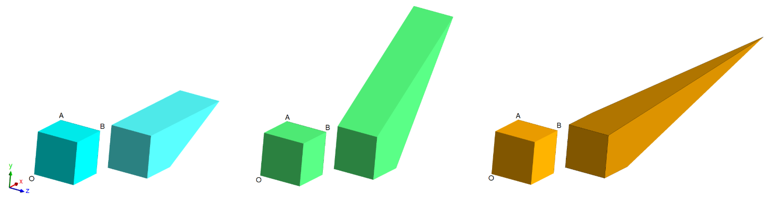
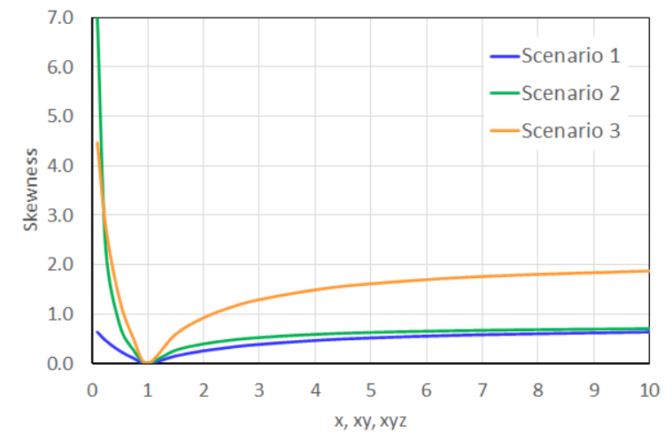
In the first scenario, the segment AB is moved along the x-direction; in the second scenario, the segment AB is moved along the 0xy-bisector; in the third scenario, vertex B moves along the central line of the 0xyz-trihedron. The first two scenarios also apply to a square. Figure 4.109: Skewness Values vs. Element Shape displays the skewness values as a function of the element shape dictated by the segment AB according to the selected scenario of Figure 4.108: Three Deformation Scenarios.
Use the Methods task to determine specific solution techniques that can be applied to your simulation.
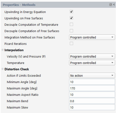
The choice of numerical methods can influence the simulation's rate of convergence as well as the solution's accuracy and stability, however, the default settings applied in the workspace are adequate most of the time.
See Methods Properties for details.
Use the Calculation Activities task to determine what, if any, activities will be performed during the calculation of the solution.
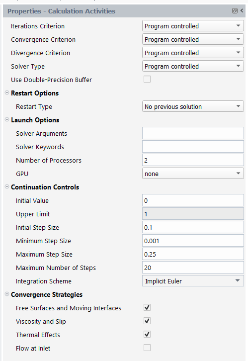
In most cases, the default settings are adequate. However, information on the AMF and AMF + secant solver types are outlined in AMF Direct Solver and AMF Direct Solver + Secant.
See Calculation Activities Properties for details.
The default solver is the algebraic multifrontal (AMF) direct solver (rather than mesh-based) where the critical variable ordering is based on the assembled equations, having the advantage of taking into account more sparsity in many systems of equations (for example, in multimode viscoelastic models where stress modes are uncoupled).
Factors are, by default, stored in memory. It is also possible to force the
storage of those factors onto disk by entering IPONDISK
for Solver Keywords. In such a case, the location on disk
is dictated by the TMP (Linux) or
TEMP (Windows) environment variable.
In many nonlinear problems, it is possible to take advantage of the system regularity between iterations in order to factorize the system matrix only from time to time. This is referred to as the secant, or modified Newton, iterative process. This technique is known to work in most problems with potentially significant savings (as the CPU-dominant system solution step is performed less frequently and system assembly can be done at a reduced cost), however, in very rare cases, the secant iteration may direct iterations along a wrong path, therefore, this option is not the default. Note that this technique requires slightly more disk space for storing the factors than is the case for the pure Newton-Raphson scheme, so do not expect memory savings from this technique.
The Fluent Materials Processing workspace provides the MUMPS (Multifrontal Massively Parallel Solver) for shared memory.
You can specify the MUMPS solver within the Calculation Activities properties panel by selecting MUMPS direct solver from the Solver Type drop-down list.
MUMPS is a package for solving systems of linear equations of the form Ax=b, where A is a square sparse matrix. As the AMF solver, MUMPS implements a direct method based on a multifrontal approach which performs a Gaussian factorization
 | (4–21) |
where  is a lower triangular matrix and
  an upper triangular matrix.
Similarly to the AMF solver, the system is solved in three main steps:
Analysis
During the analysis, Mumps creates the elimination tree (variables elimination order) and estimates the number of operations and the memory necessary for the factorization and the solution.
Factorization
The factorization computes the
 and
and  matrices and stores them in double precision. They can
be stored in core memory or on disk.
matrices and stores them in double precision. They can
be stored in core memory or on disk. Solution
The solution is obtained through a forward elimination step:

(4–22)
followed by a backward elimination step

(4–23)
In terms of continuation/transient steps and iterations, the AMF and MUMPS solvers behave similarly. Extensive testing on approximately one thousand cases has shown that any convergence issues only occurred in about 1% of cases. For most cases, the MUMPS solver is recommended.
If the CPU time is dominated by the system resolution (large 3D extrusion problems or large 3D problems with contact), MUMPS can reduce the CPU time by about 25 - 30% with peak value up to 50%. The additional memory requirement can reach 200 - 300%. If Out-Of-Core storage is invoked, this additional memory requirement is only 10 to 20% with a CPU penalty of a few percent on fast disks.
If the CPU time is not dominated by the solver (2D problems, problems with contact evaluation, problems with mesh refinement) the benefit of MUMPS in term of CPU is around 10% with peak value up to 20%. Usually, for these kind of problems, the memory is not an issue.
To activate the Out-Of-Core (OOC) storage of the factor's matrix, that is, storage on disk, you can enter the following command for Solver Keywords within the Launch Options group of the Calculation Activities panel
MUMPS_AUTO_SWITCH_OOC_MEMORY NNN
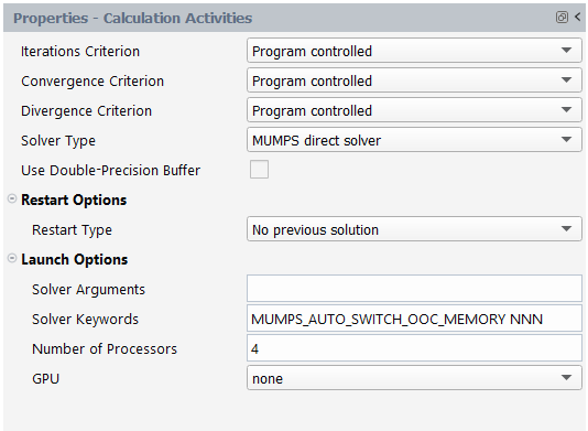
where NNN is the in-core (IC) memory value (in MB)
to be used before switching to OOC memory for the MUMPS solver. For example,
entering MUMPS_AUTO_SWITCH_OOC_MEMORY 500 specifies
the MUMPS solver to use 500 MB of in-core memory before switching to
out-of-core memory. If the estimated memory evaluated by MUMPS is greater
than the value of NNN, then the Out-Of-Core storage
will be used by MUMPS.
Just as for the AMF Direct Solver, the secant iterative process can be selected for the MUMPS solver. The secant approach has the same advantages and disadvantages with MUMPS as with AMF, as described in AMF Direct Solver + Secant. You can specify the MUMPS solver + secant within the Calculation Activities properties panel by selecting MUMPS direct solver + secant from the Solver Type drop-down list.
Use the Outputs task properties (Figure 4.112: Properties of Outputs) to configure any output-specific settings that will accompany the solution.
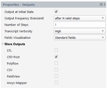
In most cases, the default settings are adequate.
See Outputs Properties for details.
Use the Monitors task properties (Figure 4.113: Properties of Monitors) to configure any monitors that will describe the solution's convergence.
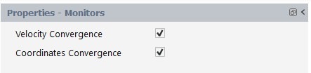
Depending on the type of simulation (blow molding, extrusion, etc.) some convergence criteria are already enabled by default.
In most cases, the default settings are adequate.
See Monitors Properties for details.
Once you have set up the simulation, use the Run Calculation task in the Outline View to access the Figure 4.114: Properties of Run Calculation.
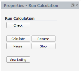
This task includes options to:
Check the setup of your simulation.
Click the Check button to check the setup of your simulation. Any relevant messages are displayed in the console window, and you are notified if and when the solver can be started.
Calculate a solution.
Once you have checked your simulation setup, click the Calculate button to start the solver.
Interrupt the calculation.
Once you have started your calculation, click the Interrupt button to pause the solver.
Stop the calculation.
Once you have started your calculation, click the Stop button to halt the solver.
View Listing of your calculations.
Once your calculation is complete, click the View Listing button for instructions about viewing the solution transcript, available as a docked tab next to the graphics window.