Depending on your requirements, there are several types of simulations you can perform using the workspace.
- 4.5.1. Modeling Internal Flows
- 4.5.2. Modeling the Prediction of Extrudate Shape (Direct Extrusion)
- 4.5.3. Modeling the Determination of Die Lip Shape (Inverse Extrusion)
- 4.5.4. Modeling Blow Molding and Thermoforming
- 4.5.5. Modeling Pressing
- 4.5.6. Modeling Compounding and Mixing
- 4.5.7. Modeling Film Casting
- 4.5.8. Modeling Filling
- 4.5.9. Modeling Foaming
- 4.5.10. Modeling Coextrusion
- 4.5.11. Modeling Fiber Spinning
- 4.5.12. Radiation model
The simulation of an internal flow is probably one of the easiest applications of the Fluent Materials Processing workspace. Here, one typically calculates velocity, pressure, possibly temperature fields which develop in the flow in a non-deformable closed domain or in a confined flow through a domain with entry and exit.
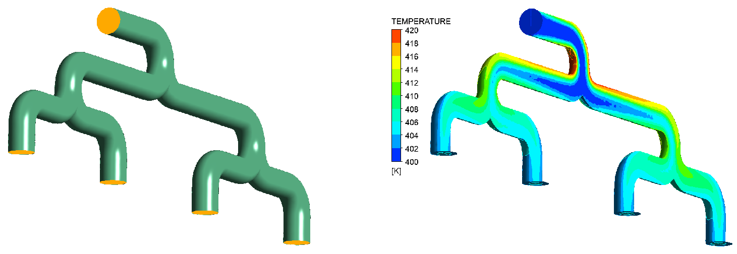
Figure 4.7: An Example of Internal Flow illustrates internal flow in a confined domain with one entry and four exits, with the geometry (left) and typical temperature distributions on the inlet, outlets, and central symmetry plane (right). The flow domain is a distributor with one entry on the top and four exits below. In general, such a calculation provides useful output such as, but not limited to, pressure and temperature. Important components are the following:
the geometry with at least one zone and at least one boundary for the flow in a closed domain, and at least three boundaries otherwise (inlet, wall, exit),
appropriate material data,
boundary or operating conditions, such as flow rate, behaviour along the die wall, condition at the exit.
Rheological Models
For setting up the calculation of an internal flow, all generalized Newtonian fluid models, differential viscoelastic models, as well as the simplified viscoelastic model can be invoked, under both isothermal ands non-isothermal conditions. However, the confined character of the flow is such that viscoelasticity can often be discarded, and you can focus on the viscosity properties. Default values are assigned to the several parameters, but you are encouraged to confirm the settings. There are also material data files available in the Extrusion and Miscellaneous categories in the available materials library.
Domains and Boundary Conditions
The calculation domain must contain at least one zone.
As can be seen in Figure 4.7: An Example of Internal Flow, the calculation domain for the confined flow with entry and exit a is surrounded by at least three boundaries:
the inlet where a flow rate is usually assigned,
the fixed die wall where slipping can be specified, and
the exit of the calculation domain.
Sometimes, additional boundaries are needed: this is typically the case when symmetry planes exist and need to be taken into account, or for example, as suggested in Figure 4.7: An Example of Internal Flow, when there are several exits.
Additional Modeling Features
There are some possibilities for expanding the model used for calculating an internal flow.
Thermal effects can be considered and requires selecting appropriate material data such as thermal conductivity, heat capacity, as well as possible temperature dependence of material properties. Thermal effects, including possible conjugated heat transfer with the solid die, also requires assigning thermal boundary conditions and specifying appropriate temperature initialization.
Restrictors can be embedded in the die, but they cannot be combined with viscoelasticity.
Foaming is not relevant here.
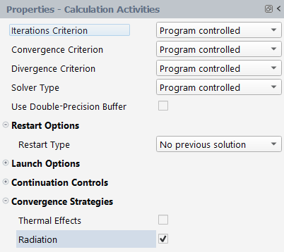
Convergence Strategies
The main sources of non-linearity in the setup for the calculation of an internal flow originate from the material properties and possibly from thermal effects. For facilitating the calculation, convergence strategies have been implemented and made available and you must select them in accordance with the setup. While a convergence strategy for rheology and slipping is often recommended, you can also invoke convergence strategies for thermal flows.
Additional Information
There are additional resources for exploring this type of simulation:
To use a template to calculate internal flow, see Using the Internal Flow Template.
To use a wizard to calculate internal flows, see Using the Simple Internal Flow Wizard.
For an example of internal flow, see Thermal Simulation of the Internal Flow of a Fluid in a Channel with One Entry and Four Exits.
The prediction of extrudate shape (also known as direct extrusion) is one of the flagship applications of the Fluent Materials Processing workspace. Most often, it concerns materials such as molten polymer or uncured rubber. The definition of this application is easy: considering a die with given shape and dimensions, it provides information on the extrudate, based on material properties and boundary conditions.
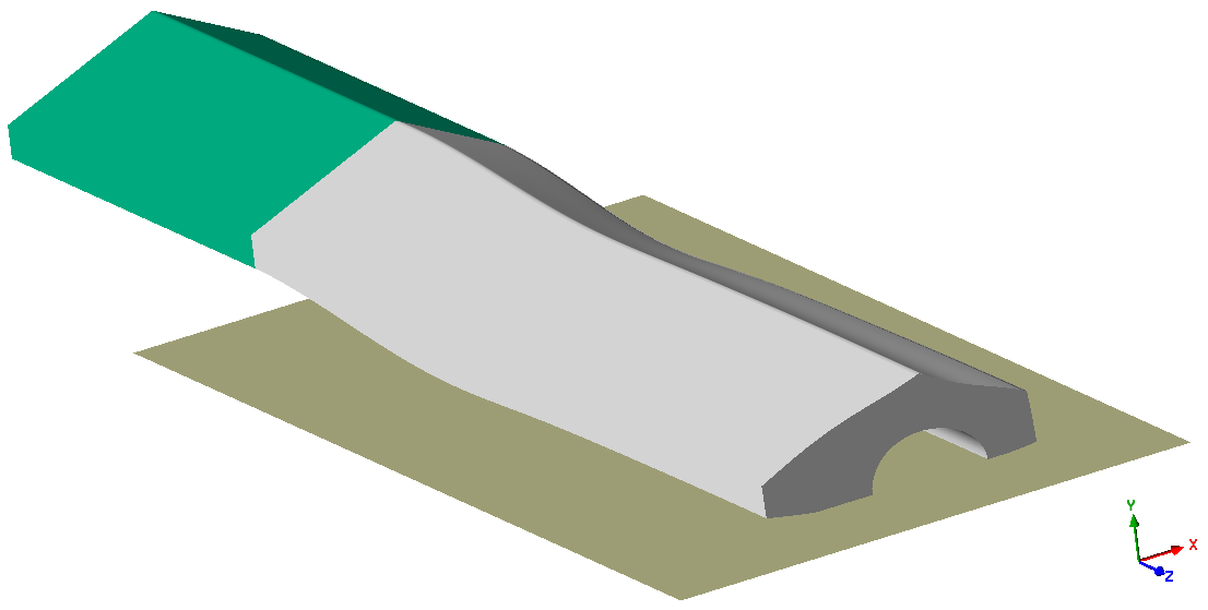
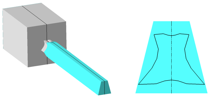
Figure 4.8: An Example of Direct Extrusion illustrates a realistic model for the simulation of an extrusion flow assisted by a conveyor belt. From left to right, the melt (grey) enters the die channel (green), flows through the channel, exits the die, and is subsequently conveyed by a belt (brown) on which it lays due to the effect of gravity. It is important to mention that the use of a conveyor belt is not mandatory, while gravity does not necessarily play a visible role. All of these are more or less case specific, however, the important components are the following:
the geometry contains at least two zones (one for the flow within the die, one for the extrudate) and at least four boundaries (inlet, wall, free surface, exit),
appropriate material data,
boundary or operating conditions, such as flow rate, behaviour along the die wall, condition at the exit.
The following components are important to consider for this type of simulation:
Rheological Models
For setting up the prediction of extrudate shape, all generalized Newtonian fluid models, differential viscoelastic models, as well as the simplified viscoelastic model can be invoked, under both isothermal and thermal conditions. Default values are assigned to the several parameters, but it is always a good idea to check them. There are also material data files available in the Extrusion and Miscellaneous categories in the available materials library.
Domains and Boundary Conditions
The calculation domain must contain at least two zones. One zone is needed for the calculation of the flow within the die, another zone is needed for the calculation of the extrudate that deforms from the die exit until the exit of the calculation domain. A mesh deformation algorithm is applied on this latter zone.
As can be seen in Figure 4.8: An Example of Direct Extrusion, the calculation domain is surrounded by at least four boundaries:
the inlet where a flow rate is usually assigned,
the fixed die wall where slipping can be specified,
the outer border of the extrudate where free surface conditions are imposed, and
the exit of the calculation domain. On this latter border, a take-up force or velocity can be imposed. A stress free condition is also possible.
Sometimes, additional boundaries are needed. This is typically the case when symmetry planes do exist and are taken into account. This can also be the case when you want to define a moving wall that mimics a wire or a metal insert, for example, in a coating process.
Additional Modeling Features
There are some possibilities for expanding the model used for calculating a direct extrusion.
The present simple model for extrudate shape prediction can be expanded by adding a few more features, such as foaming or thermal effects. Thermal effects requires selecting appropriate material data such as thermal conductivity, heat capacity, as well as possible temperature dependence of material properties. Thermal effects, including conjugated heat transfer with the solid die, also requires assigning thermal boundary conditions and specifying appropriate temperature initialization.
Restrictors can be embedded in the die, but they cannot be combined with viscoelasticity and foaming.
Specific features can be selected for the extrudate. A take-up force or velocity can be assigned at the exit of the computational domain. For small profiles, that is, when gravity effects can be neglected, it is often useful to invoke the free jet stabilization when the profile lacks symmetry. For heavier profiles, that is, when gravity effects play a visible role, it is a good idea to define a conveyor belt or a roller conveyor, as is most likely present in the actual process.
Convergence Strategies
A model for extrudate shape prediction can involve several non-linearities originating from the geometry, the rheology and the boundary conditions. For facilitating the calculation, convergence strategies have been implemented and made available. While a convergence strategy for free surfaces and moving interfaces is often recommended, you can also invoke convergence strategies for thermal flows, rheology and slipping, and/or foaming.
Additional Information
There are additional resources for exploring this type of simulation:
To use a template to calculate the prediction of extrudate shape, see Using the Extrusion Template.
To use a wizard to calculate the prediction of extrudate shape, see Using the Simple Direct Extrusion Wizard.
For a tutorial that demonstrates the prediction of extrudate shape, see 3D Polymer Extrusion.
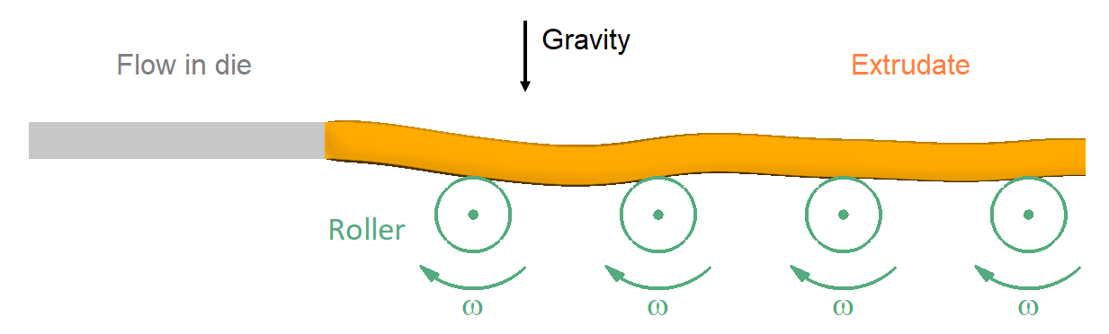
Some industrial extrusion applications involve the use of conveyor devices. This is typically the case for profiles whose dimensions and weight require such a guiding device. An illustrative example is the rubber tire tread extrusion process: downstream of the die exit, the profile is sustained by a series of rotating conveyor cylinders or by a moving conveyor belt, at a speed that matches the extrusion line speed.
Some geometric details of the conveyor belt or conveyor cylinders are discarded: instead, they are defined in simple geometric terms and by their role in the extrusion process, or more precisely, within the scope of the extrusion model. Since such a device (either a belt or roller) guides the extrudate profile at a given location and at a given speed, it will be described by means of those quantities. On one hand, a conveyor is represented by a plane defined by a point and an outward direction perpendicular to it, that is, oriented towards the extrudate; while a velocity is assigned. On the other hand, a conveyor roller is represented by a cylinder defined by a radius, an axis direction and a point of the axis, while a rotating velocity is assigned; quite obviously, several conveyor rollers can be involved. By the way, the workspace allows to define a Roller Conveyor that is a series of identical rollers having the same angular velocity.
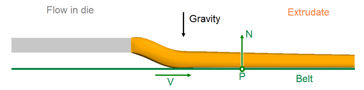
Figure 4.9: An Extrusion Process Involving a Conveyor Belt illustrates a basic extrusion case involving the use of a conveyor belt. As suggested, the conveyor belt is a plane described by a conveniently selected point P, an outward normal direction N to the plane and a velocity V.
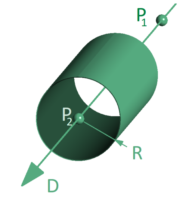
Similarly, Figure 4.10: An Extrusion Process Involving Conveyor Rollers illustrates
an extrusion case involving a series of rollers. A conveyor roller is a cylinder
defined by its radius R, two points P1
and P2 specifying an oriented axis D,
as well as a (signed) angular velocity  around the axis.
In addition, Figure 4.11: Perspective View of a Roller with Geometric Parameters illustrates the geometric details of the roller.
From the deformation of the extrudate as suggested in both Figure 4.9: An Extrusion Process Involving a Conveyor Belt and Figure 4.10: An Extrusion Process Involving Conveyor Rollers, it is understood that gravity plays a role in the process: the guiding device will prevent further downward deformations. Also, the extrudate is obviously pulled at the end of the computational domain: a velocity must be imposed at the exit section, and this is anyway preferable than imposing a normal force that is a priori unknown. Some guiding devices purposely drag the extrudate, in which case the relative tangential velocity between the extrudate and the device is controlled by a slipping coefficient, after the fashion of the Navier’s slipping law. A frictionless guiding device (for example, an air cushion) is a specific case where the friction coefficient is set to zero.
For steady-state extrusion simulations that do not involve any implicit constraints on the extrudate (for example, plane of symmetry, slip conditions, or guiding devices), the Fluent Materials Processing workspace will apply a global displacement constraint if the problem satisfies certain conditions, which are described later in this section.
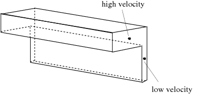
To avoid excessive global displacement, the model allows the addition of a force and a torque on the free jet (or a portion of it). The computed force and torque can be interpreted as those produced by a guide used to prevent deviations in the extrudate shape. In a well-balanced die, the deviation of the extrudate is small and the force and torque are also small. An unbalanced die, however, will have very large deviations. Consider the unbalanced die illustrated in Figure 4.12: Flow Through an Unbalanced Die.
The extrusion of such a profile leads, in general, to a large deviation in the extrudate due to the differences in velocity. The deviation of the jet is produced by a nonzero average transverse velocity (ATV) in the cross-section (for example, at the die exit).
To avoid large displacements (translation and rotation) of the free jet, the Fluent Materials Processing workspace applies a force and a torque on all or part of the extrudate, if the problem satisfies certain conditions described later in this section.
The force  and torque
  actually act as distributed quantities in the equation of
motion. The values of the force and torque components are computed by the
Fluent Materials Processing workspace precisely so as to obtain a zero averaged transverse
velocity (or rotation). When the large displacements are avoided,
convergence of the solution becomes much easier.
actually act as distributed quantities in the equation of
motion. The values of the force and torque components are computed by the
Fluent Materials Processing workspace precisely so as to obtain a zero averaged transverse
velocity (or rotation). When the large displacements are avoided,
convergence of the solution becomes much easier.
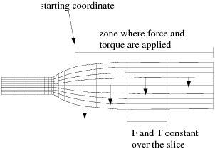
The mesh is sliced along the extrusion direction according to the definition of the mesh deformation algorithm. On each node slice (that is, group of all nodes belonging to the same slice), the force and torque are assumed to be constant, as shown in Figure 4.13: Sliced Domain with Force and Torque.
Furthermore, the component of the force in the flow direction and the component of the torque in the transverse direction have imposed values of zero. Since the force and torque are constant in each slice, their effect on the shape of the extrudate section is small.
The following limitations apply to the free jet stabilization:
It is available only for non-axisymmetric extrusion problems. (Axisymmetry implicitly involves a free jet stabilization around the axis.)
The extrusion direction must be aligned with the
 ,
,  , or
, or  direction. When Optimesh 3D or streamwise mesh
deformation algorithms are used, the Fluent Materials Processing workspace will check
that the inlet and outlet sections are real planes and are
perpendicular to the
direction. When Optimesh 3D or streamwise mesh
deformation algorithms are used, the Fluent Materials Processing workspace will check
that the inlet and outlet sections are real planes and are
perpendicular to the  ,
,  , or
, or  direction.
 Optimesh, the streamwise method, the method of spines (2D) must be used as the mesh deformation algorithm, so that slicing is available.
Although the Elastic deformation method with torsion control does not formally require a sliceable mesh, the constraint on the free jet requires such a mesh. Hence, you will be able to apply free jet stabilization when using this mesh deformation algorithm, if the mesh is at least sliceable. If the mesh is not sliceable on the extrudate, the Fluent Materials Processing workspace stops on an error message.
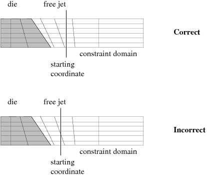
The plane passing by the relative starting coordinate and perpendicular to the extrusion direction must not cross any slice (that is, the force or torque must either apply on an entire slice or not apply at all on the slice). If this condition is violated, the solver will not converge. Figure 4.14: Constraint on the Starting Coordinate illustrates correct and incorrect positions for the starting coordinate.
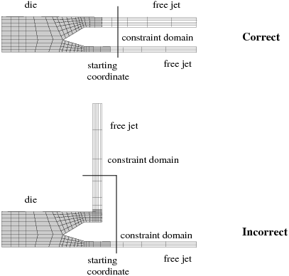
For multiple-jet simulations, the extrusion direction must be the same for all jets. The force and torque on each jet will, however, be computed separately. Figure 4.15: Constraint on Multiple-Jet Problems illustrates multiple-jet problems for which the constraint can and cannot be applied.
The free jet stabilization is not compatible with velocity boundary
conditions on the extrudate (for example, plane of symmetry:  ; belt conveyor:
  ,
,  ). These velocity conditions are sufficient to avoid global
displacements, so no additional constraints are required. For this reason,
some force or torque components can be set to zero. Table 4.9: Force and Torque Components for Geometries and Boundary
Conditions
identifies the force and torque components for different cases as computed
(C), equal to zero (0), or not computed (N) because they are incompatible
with the boundary conditions. In this table, the flow direction is
). These velocity conditions are sufficient to avoid global
displacements, so no additional constraints are required. For this reason,
some force or torque components can be set to zero. Table 4.9: Force and Torque Components for Geometries and Boundary
Conditions
identifies the force and torque components for different cases as computed
(C), equal to zero (0), or not computed (N) because they are incompatible
with the boundary conditions. In this table, the flow direction is
 for non-axisymmetric 2D geometries, and
  for axisymmetric and 3D geometries.
The table tells you which component of the force or torque will be non-zero when the free jet stabilization is used. If you specify an inconsistent constraint, the Fluent Materials Processing workspace will warn you.
Table 4.9: Force and Torque Components for Geometries and Boundary Conditions
| Geometry | Boundary Conditions |  |  |  |  |  |  |
|---|---|---|---|---|---|---|---|
| 2D axisym (Figure 4.16: 2D Geometries a) | line of axisymmetry | N | – | 0 | – | – | – |
| 2D planar (Figure 4.16: 2D Geometries b) | no plane of symmetry | C | 0 | – | – | – | – |
| 2D planar (Figure 4.16: 2D Geometries c) | plane of symmetry,  | N | 0 | – | – | – | – |
| 2D planar (Figure 4.16: 2D Geometries d) |  , ,  | N | – | – | – | – | – |
| 3D (Figure 4.17: 3D Geometries a) | no plane of symmetry | C | C | 0 | 0 | 0 | C |
| 3D (Figure 4.17: 3D Geometries b) | one plane of symmetry,  | C | 0 | 0 | 0 | 0 | 0 |
| 3D (Figure 4.17: 3D Geometries c) | two planes of symmetry,  or or  | 0 | 0 | 0 | 0 | 0 | 0 |
This information must come either from your knowledge of the process being modeled or from your observation of large deviations in a previous simulation.
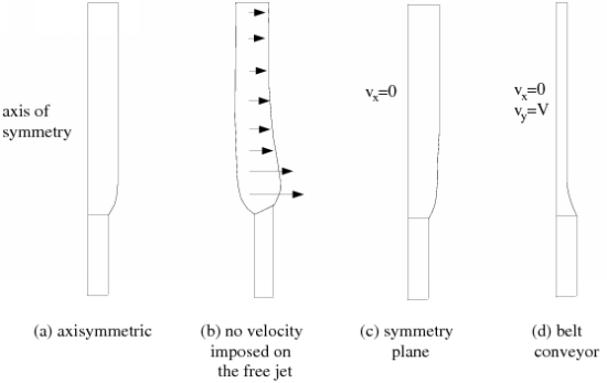
For 2D geometries, there is no torque and
 or
or  is zero. Axisymmetric geometries (Figure 4.16: 2D Geometries a) are incompatible with the constraint on
global displacement.
is zero. Axisymmetric geometries (Figure 4.16: 2D Geometries a) are incompatible with the constraint on
global displacement. For a 2D geometry without velocity boundary conditions on the free jet (Figure 4.16: 2D Geometries b), there is only one component of force that is computed. 2D geometries with a symmetry plane (Figure 4.16: 2D Geometries c) or with normal (to the extrusion axis) velocity imposed (Figure 4.16: 2D Geometries d) are incompatible with the constraint on global displacement.
For 3D geometries without velocity boundary conditions on the free jet (Figure 4.17: 3D Geometries a), the transverse components of the force are computed in order to avoid the displacement in the transverse direction, and the force component in the flow direction is equal to zero; the torque components in the flow direction is computed in order to avoid extrudate rotation, and the other torque components are equal to zero.
For 3D geometries with one plane of symmetry (Figure 4.17: 3D Geometries b), extrudate rotation is not possible, so the torque is not taken into account. Since displacement in the direction perpendicular to the symmetry plane is not allowed, the force in this direction is imposed to be zero.
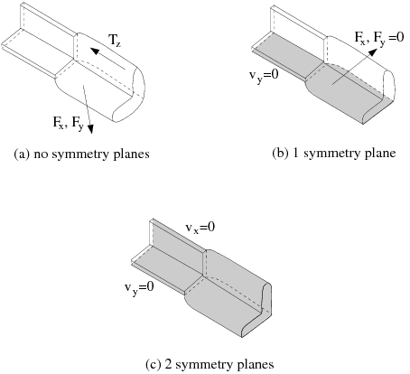
For a 3D geometry with two planes of symmetry or other velocity boundary conditions (Figure 4.17: 3D Geometries c), the transverse and rotation displacements of the free jet are not possible, so the force and torque are not taken into account.
The Fluent Materials Processing workspace detects these situations automatically and sets the appropriate force and torque components to zero. If you try to use the constraint on global displacement when it is incompatible with the boundary condition, the Fluent Materials Processing workspace will inform you of the incompatibility in an error message.
The determination of die lip shape is another application of the Fluent Materials Processing workspace, also known as inverse extrusion. This application most often concerns materials such as molten polymer or uncured rubber. It can be defined as follows: consider a given extrudate profile with specific dimensions, the application provides indications toward the design of die lips needed, based on material properties and boundary conditions.
The left hand side of Figure 4.18: Example of Inverse Extrusion displays a sketch of a realistic model for the determination of die lip shape for the extrusion of a given profile. From left to right, the melt (blue) enters the die channel (grey), flows through the channel, and exits the die (symmetry is suggested by the black line). The right hand side of Figure 4.18: Example of Inverse Extrusion displays a comparison between the required extrudate shape (blue) and the calculated die lips (black line). All this is case specific, and there are indeed several possible topological scenarios when determining the die lip shape: calculation of a constant die land only, of a converging die land only, a combination of both, etc. Important components, however, are the following:
the geometry contains at least two zones (one for the flow within the die, one for the extrudate) and at least four boundaries (inlet, wall, free surface, exit),
appropriate material data,
boundary or operating conditions, such as flow rate, behaviour along the die wall, condition at the exit.
Rheological Models
For setting up the prediction of die lip shape, all generalized Newtonian fluid models, differential viscoelastic models, as well as the simplified viscoelastic model can be invoked, under isothermal or thermal conditions. Default values are assigned to the several parameters, but it is always a good idea to check them. There are also material data files available in the Extrusion and Miscellaneous families in the Library of Materials.
Domains and Boundary Conditions
The calculation domain must contain at least two zones. One zone is needed for the calculation of the flow within the die, and another zone is needed for the calculation of the extrudate which deforms from the die exit until the exit of the computational domain. Zones can be added to the die when a converging section and a fixed section are involved. A mesh deformation algorithm is applied on all but the fixed section.
As seen in Figure 4.18: Example of Inverse Extrusion, the calculation domain is surrounded by at least four boundaries:
the inlet where a flow rate is usually assigned,
the fixed die wall where slipping can be specified,
the outer border of the extrudate where free surface conditions are imposed, and
the exit of the calculation domain. On this latter border, a take-up force can be imposed. A stress free condition is also possible.
Sometimes, additional boundaries are needed, for example, when symmetry planes do exist and are taken into account. This can also be the case when one wants to define a moving wall which mimics a wire or a metal insert, for example, in a coating process.
Additional Modeling Features
The present simple model for determining die lip shape can be expanded by adding a few more features. Foaming can be included. Thermal effects, including conjugated heat transfer with the solid die, can be considered. This requires selecting appropriate material data such as thermal conductivity, heat capacity, as well as possible temperature dependence of material properties, in addition to assigning thermal boundary conditions and specifying appropriate temperature initialization.
Specific features can be selected for the extrudate. A take-up force can be assigned at the exit of the computational domain. Also, when the profile lacks symmetry, it is useful to invoke the free jet stabilization.
Restrictors can be embedded in the fixed section of the die only, but they cannot be combined with viscoelasticity and foaming. Eventually, the determination of die lip shape cannot be combined with the use of guiding devices.
Convergence Strategies
A model for determining the die lip shape involves several non-linearities originating from the geometry, the rheology and the boundary conditions. For facilitating the calculation, convergence strategies have been implemented and made available. In addition to a recommended convergence strategy for free surfaces and moving interfaces, you can also invoke convergence strategies for rheology and slipping, for thermal flows and for foaming. The required convergence strategies are automatically activated when using a wizard; when using a template or performing a manual setting, you must select convergence strategies in accordance with the setup.
Additional Remarks
To some extent, this virtual analysis may replace a first real experiment. The solution quality is subjected to several factors, such as the available data, the assumptions made, etc. As for many applications, common sense and validations are certainly welcome in the design process.
Additional Information
There are additional resources for exploring this type of simulation:
To use a template for applications that determine die lip shape, see Using the Extrusion Template.
To use a wizard for applications that determine die lip shape, see Using the Simple Inverse Extrusion Wizard.
For a tutorial that demonstrates determining die lip shape, see 3D Inverse Extrusion.
Blow molding is a manufacturing process for forming hollow polymer parts.
There are two main types of blow molding: extrusion blow molding and injection blow molding. In the first process, molten polymer is extruded into a hollow tube, a parison. This tube is closed by pinching it in a mold and is finally blown into the desired hollow part. In the second process, a preform is injection molded and transferred into another mold in which it is inflated into the final article shape. When the inflation of the preform is assisted by a plunger, the process is also called injection stretch blow molding.
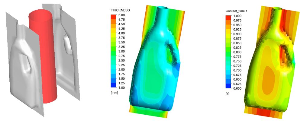
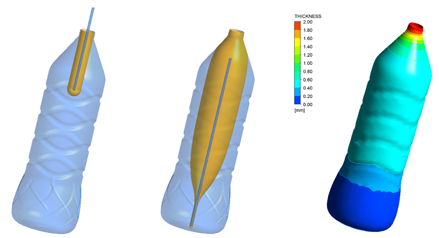
Figure 4.19: Simple Model for an Extrusion Blow Molding Application displays a simple model for extrusion blow molding simulation. Likewise, Figure 4.20: Simple Model for an Injection Stretch Blow Molding Application displays an injection stretch blow molding application.
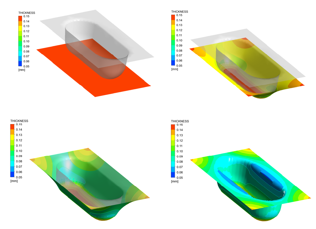
Thermoforming refers to the forming of a polymer sheet into a 3D shape by using a mold, heat, vacuum/pressure and/or a plunger. Thermoforming is used in a wide variety of applications, such as cups, blisters, trays and covers, packaging items, dash panels, refrigerator liners, etc. Figure 4.21: Simple Model for Thermoforming Application displays a simple model for the thermoforming of a pharmaceutical blister.
Blow molding and thermoforming simulations make use of the same tools: a shell model for polymer parison/sheet, contact detection when the fluid meets the mold and/or the plunger, the large deformations of the fluid material that renders mesh adaption quite necessary, the geometrical details of the mold that must be captured and the thermal effects.
This section focuses on methods using the shell element that can be used when the thickness of the fluid layer is small compared to other dimensions. When this assumption is not valid or for 2D cases, standard volume elements must be used (in such cases, see Modeling Pressing).
Rheological Models
Since stretching is the main deformation of the polymer parison/sheet, you should consider a model that exhibits some amount of strain hardening, or at least no thinning in extension. So, the simplest rheological model is a pure Newtonian model with a constant viscosity. A second option is a multi-mode integral viscoelastic model. An attractive option is the use of a strain-dependent viscosity while an orthotropic material model can also be used when the polymer is reinforced by oriented fibers. In all cases, isothermal and thermal conditions can be defined
Domains and Boundary Conditions
In the simplest configuration, two zones are sufficient, one for the fluid and one for the mold. For more complex cases, several molds and/or plungers can be defined.
For the boundaries, a single boundary for the fluid domain might be sufficient but additional boundaries must be defined for planes of symmetry.
A single boundary is usually sufficient for a mold or a plunger.
Additional Modeling Features
In many cases, the motion of the plunger(s) is not constant and expressions must be used to define the velocity components of the displacement as function(s) of time (see Using Expressions in the Workspace for more information about expressions).
In some cases, especially injection stretch blow molding ones, it is necessary to allow contact release. This makes the fluid able to detach from the plunger.
It is also possible to define a fluid sheet/parison made of several layers. Each layer is made of a different material and has its own specific thickness. The fluid shell's behavior is then a result of the combination of the different layers.
Thermal effects can be considered, and require additional material data as well as assigning thermal boundary conditions and specifying temperature initialization. Heat transfer with the mold(s) and plungers is also possible.
Related Notes
As a mold/plunger is represented by a shell, it is important to specify on which side of this shell the solid body is located.
As the fluid domain is a shell in the 3D space, planes of symmetry must be defined by specifying their normal.
As for any simulation involving large deformations, adaptive meshing is highly recommended. In the case of shells, the mesh adaptation is performed via subdivision of the original elements.
Additional Information
There are additional resources for exploring this type of simulation:
To use a template for the blow molding / thermoforming applications, see Using the Blow Molding & Thermoforming Template.
For a tutorial that demonstrates injection stretch blow molding, see Injection Stretch Blow Molding (ISBM).
Pressing is a forming process where a force is applied to a material to deform it to match the size and shape of a die usually consisting of a fixed mold and a moving plunger. Pressing is much used to produce glassware.
Figure 4.22: Example of Pressing displays a sketch of a simple model for glass pressing simulation, where two planes of symmetry have been taken into account.
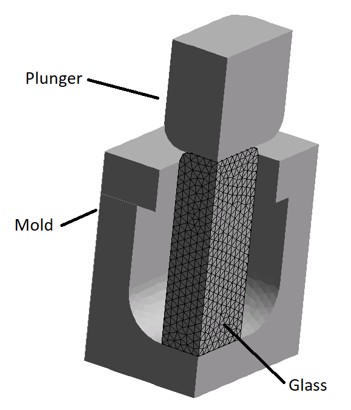
The important components of such simulations are the contact detection when the fluid meets the mold and/or the plunger, the large deformations of the fluid material that renders mesh adaption quite necessary, the geometrical details of the mold that must be captured and the thermal effects, especially in the case of glass.
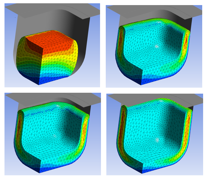
Figure 4.23: Time Evolution of the Glass Blob With Contours of Velocity displays the fluid domain at four different instants of the pressing process. The velocity contours allows you to observe that the fluid is pushed down in a first stage but is pushed up between the plunger and the mold in a second stage. Note the mesh adaptation that allows you to cope with the large deformations of the material.
Rheological Models
For setting up the simulation of pressing, all generalized Newtonian fluid models may be used, under isothermal and thermal conditions. Differential viscoelastic models are not recommended and would lead to very important calculation times.
Domains and Boundary Conditions
The calculation domain usually contains three zones, one for the fluid, one for the mold, and one for the plunger. If several molds and/or plungers are necessary, a zone must be defined for each of them.
For the boundaries, a single boundary for the fluid domain might be sufficient but additional ones must be defined for planes of symmetry.
A mold or a plunger usually has two boundaries, one for the contact with the fluid, and a second one for the rest of its border. A larger number of boundaries is nevertheless permitted if you want to define several contact boundaries or to clearly identify planes of symmetry and/or different thermal boundary conditions.
In many cases, the motion of the plunger(s) is not constant and expressions must be used to define the velocity components of their displacement as functions of time.
In some cases, it is necessary to allow contact release. This makes the fluid able to detach from the mold/plunger.
In addition or in replacement of the plunger, a pressure can be applied to deform the gob of fluid. This allows you to simulate blow molding with volume elements.
Thermal effects can be considered, and require additional material data as well as assigning thermal boundary conditions and specifying temperature initialization. Heat transfer with the mold(s) and plungers is also possible.
Additional Remarks
Volume conservation is activated by default. This guarantees that, despite the numerous remeshings, the mass of fluid remains constant.
To assist in keeping a suitable mesh, refinement zones can be defined. They can be boxes or spheres in which the size of elements are prescribed, they also can be a refinement along boundaries where geometrical details must be captured. In the latter case, the required element size can be function of the distance to contact or function of the curvature of the contact surface.
Refinement along boundaries are especially useful in non-isothermal calculations where thermal boundary layers must be captured
Additional Information
There are additional resources for exploring this type of simulation:
To use a template for pressing applications, see Using the Pressing Template.
For an example that demonstrates tire molding, see Reinforcements and Pantographing in Rubber Tire Molding.
Mixing and compounding are typically internal flows which involve moving parts. Apart from a few situations, the motion of the moving part is such that the geometric configuration evolves with time. Typical examples are stirring tanks, single- and twin-screw extruders, pistons. With changing geometric configuration, the flows are intrinsically transient, with or without entry and exit. With a setup for mixing and compounding, one typically calculates velocity, pressure, possibly temperature fields which develop in a confined domain that changes with time: an appropriate treatment of overlapping meshes is applied for easily generating the changing flow domain.
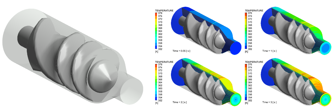
Figure 4.24: Example of a Geometry for a Single-screw Extruder displays a sketch of a domain for the transient calculation of the flow of a viscous material in a short single screw extruder (left) and a transient temperature field at four instances (right). In the suggested model, the barrel is fixed while the screw rotates with an angular velocity of 60 rpm (or 2π rad/s). In general, such a calculation provides useful output such as, but not limited to, pressure field and temperature rise. Important components are the following:
the geometry with at least one fluid zone and at least one moving part, and at least one boundary for a closed domain and three boundaries otherwise (inlet, wall, exit),
appropriate material data,
boundary or operating conditions, such as flow rate, behaviour along the die wall, behaviour on the moving part.
Rheological Models
For setting up the calculation of mixing and compounding flow, all generalized Newtonian fluid models can be invoked, under both isothermal and thermal conditions. Default values are assigned to the several parameters, but it is always a good idea to check them. There are also material data files available in the Extrusion and Miscellaneous families in the Library of Materials.
Domains and Boundary Conditions
The calculation domain must contain at least two zones, one for the fluid and one for the moving part. Multiple moving parts are possible, and the motion of each individual part is described as a combination of rotation and translation. The behavior of the fluid along the wall of the moving part can be specified.
As shown in Figure 4.24: Example of a Geometry for a Single-screw Extruder, the calculation domain for the flow domain for the single-screw extruder is surrounded by at least three boundaries:
the inlet where a flow rate is usually assigned,
the fixed barrel wall where slipping can be specified,
the exit of the calculation domain, and
a possible internal boundary overlapped by the moving part.
Sometimes, additional boundaries are needed, for example, when distinct fluid behavior along walls must be specified, or when there are multiple entries or exits.
Additional Modeling Features
Thermal effects, including conjugated heat transfer with the moving part, can be considered. This requires selecting appropriate material data such as thermal conductivity, heat capacity, as well as possible temperature dependence of material properties, in addition to assigning thermal boundary conditions and specifying appropriate temperature initialization.
Adaptive Meshing
With the motion of the moving part, the geometric configuration is changing throughout the calculation, and there will never be a precise match between the discretization of zones for fluid and moving part(s). Instead of selecting at the outset a very fine discretisation for the fluid zone, it is more efficient to invoke the adaptive meshing, and to specify a refinement condition in the vicinity of the transition between the zones for fluid and moving part(s). Refinement is based on element subdivision.
Additional Information
To use a template for mixing and compounding applications, see Using the Compounding & Mixing Template.
For a tutorial that demonstrates compounding and mixing, see Mesh Superposition Technique.
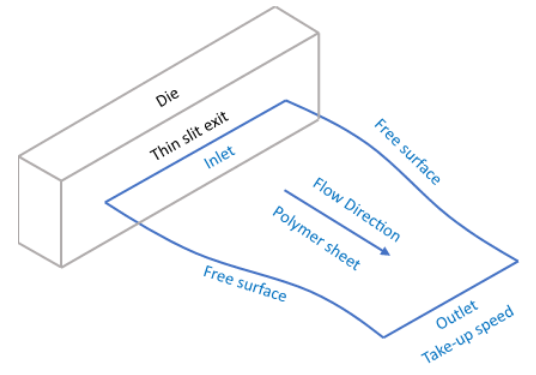
The film casting process is an important industrial continuous process to produce polymer films, films that can be made of several layers. As shown in Figure 4.25: Example of Film Casting, the molten polymer is extruded in a film through the thin slit of a flat die. The film contains two free surfaces and is then drawn in the flow direction by a higher take-up speed. This causes film width reduction and film edge thickening (so called “neck-in” and “dog-bone” effects), respectively. Both effects must be suppressed since they reduce process productivity.
A film has a thickness that is several orders of magnitude smaller than its other dimensions. It is also assumed that the film is flat, so that effects due to film curvature are ignored. Consider the problem of modeling the flow between a die exit and a take-up roll, where entrance and exit effects are ignored. The problem is truly three-dimensional since the film will show necking along lateral sides as well as a thickness variation along the principal direction of stretching. However, because of the very small thickness, a 3D model would not be feasible as it would require a very large mesh, which would result in a costly computation. Instead, a special 2D model has been developed in the workspace. In this 2D model, all conservation equations are averaged throughout the third dimension (that is, the film thickness) and thickness-averaged velocity and temperature values are computed. The film thickness becomes a variable of the flow problem, governed by the mass conservation equation. Pressure is no longer a variable of the problem and is eliminated from the momentum equations. In the case of multilayer film, each layer has its own thickness variables.
Rheological Models
For setting up the simulation of film casting, all generalized Newtonian fluid models and differential viscoelastic models are available, under isothermal and thermal conditions. However, since the flow is characterized by elongation, you should consider a model that exhibits some amount of strain hardening, or at least no thinning in extension. For the viscoelastic simulation, the stresses are computed, and in the case of multilayer simulation, each layer has its own stress variables.
Domains and Boundary Conditions
The 2D calculation domain for film problem must be planar and may be composed of several cell-zones. As shown in Figure 4.25: Example of Film Casting, the calculation domain must be surrounded by at least four boundaries:
an inlet where a normal velocity, temperature and thickness are imposed,
a free surface fixed at the inlet, for the temperature, common sense suggests to impose an insulated thermal condition,
an outlet where the take-up speed and a vanishing heat flux are imposed,
a second free surface fixed at the inlet or a plane of symmetry.
Inlet, outlet and symmetry boundaries may be composed of several parts while free surface boundaries must be in one part.
For non-isothermal simulations, a cooling flux can be applied on the surface of the film.
Stress Boundary Conditions for DCPP (Double Convected Pom Pom) Viscoelastic Model in Film Casting
For the particular case of the DCPP model, care is required when imposing the boundary conditions for the viscoelastic variables at the inlet of the calculation domain. The inlet is the border where the thickness condition is imposed. There, instead of all components of the orientation tensor, you will be prompted about anisotropy described in terms of orientation and factor, as well as stretching amplitude. Imposing boundary conditions for the viscoelastic unknowns (orientation and stretching) is optional. If conditions are imposed, you will need to provide the following information:
the direction of anisotropy of the orientation tensor (x or y),
the anisotropy factor ranging between 0 (isotropic) and 1 (anisotropic),
the inlet stretching.
Multilayer Films (Coextrusion)
Some film casting applications involve several fluid layers. In view of the model, the fluid layers may overlap or be adjacent. Several cell zones are necessary if all layers are not defined on the whole computational domain. The velocity field, as well as the temperature field (for non-isothermal problems), will be uniquely defined on the computational domain, while an independent thickness field will be assigned to each fluid layer. Also, for viscoelastic model problems, an independent extra-stress tensor will be assigned to each fluid layer. The film model does not require an interface condition between layers.
Film Problems and Nonlinearity
A film flow problem is characterized by several nonlinearities, such as mesh deformation, rheology, thermal effects, and boundary conditions. Two important effects leading to convergence difficulties are the cooling of the film and a take-up speed at the outlet of the computational domain leading to strong changes in the geometry and/or in the thickness.
When the level of nonlinearities is significant, you should use a continuation scheme for the take-up speed such that the initial take-up speed equals the inlet velocity and reaches the prescribed take-up speed at the end of the continuation scheme. For non-isothermal problems with cooling flux, the cooling flux should start from zero and reach its prescribed value at the end of the continuation scheme.
Additional Information
There are additional resources for exploring this type of simulation:
To use a template for film casting applications, see Using the Film Casting Template.
For an example that demonstrates non-isothermal multilayer film casting with multi-viscoelastic modes, see Multilayer Film Casting.
The filling of a cavity by a molten polymer is a very common process of the polymer industry. The filling is a transient process where a fluid is introduced into a cavity by a number of inlets. The process stops when the cavity is filled and air expelled out of it through vents.
In order to simulate such a process, the workspace employs a technique which is inspired from the Volume of Fluid technique (VOF) model. It is based on a time-dependent approach applied on a fixed domain where the front of fluid is tracked via the calculation of a transport variable, which allows the discrimination between both filled and unfilled parts. In the region already filled, you typically calculate velocity, pressure, and possibly temperature fields which develop from the entry to the front, and this continues until the cavity is completely filled.
The implemented model formally enables the simulation of flows that would be too complicated for a deformation-based technique, and can, for example, simulate the splitting and merging of fluid fronts, under a relatively simple geometric context.
It should be noted that the VOF model is not a replacement for Arbitrary Lagrangian-Eulerian (ALE) methods in all cases. Because the VOF technique relies on partly filled cells (which means that the location of the free surface does not correspond to an element boundary), it is intrinsically less accurate than the ALE technique for flows with well defined interfaces, such as extrusion or multiple layer problems. The ALE method may be more appropriate when searching for a well defined steady-state free surface through a steady-state (or a continuation on a free surface) algorithm.
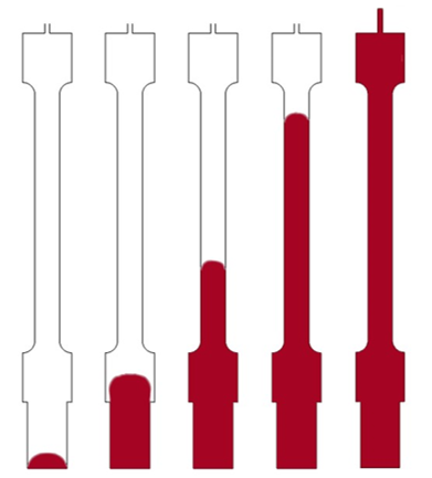
Figure 4.26: An Example of Filling displays a sketch of a domain for the calculation of the filling process together with a possible output result. The geometry is like a test sample generally used in traction tests. The flow domain has one entry at the bottom and one exit at the top. The filled part of the cavity is observed at various stages of the process, where the red area corresponds to the zone when the fluid fraction is above 0.5, indicating the area filled by the polymer (the zone with a fluid fraction below 0.5 is considered to be empty).
Important components are the following:
the geometry with at least one zone and at least three boundaries (inlet, wall, exit),
appropriate material data,
boundary or operating conditions, such as flow rate, behaviour along the cavity wall, condition at the exit.
The Volume of Fluid technique can be selected in the Calculation Type option in the General properties of the Setup. The fluid fraction is initialized to zero in the whole domain at the start (the cavity is initially empty) and set to 1 along all the inlets.
Rheological Models
All generalized Newtonian fluid models, differential viscoelastic models, as well as the simplified viscoelastic model can be invoked, under both isothermal and thermal conditions. Default values are assigned to the several parameters, but it is always a good idea to check them. There are also material data files available in the Extrusion and Miscellaneous families in the Library of Materials.
Domains and Boundary Conditions
The calculation domain must contain at least one zone.
As can be seen in Figure 4.26: An Example of Filling, the calculation domain for the flow with entry and exit is surrounded by at least three boundaries:
the inlet where a flow rate is usually assigned,
the wall where slipping can be specified, and
the exit (or vent) of the calculation domain.
Sometimes, additional boundaries are needed as this is typically the case when symmetry planes do exist and are taken into account.
Additional Modeling Features
There are actually limited possibilities for expanding the model used for calculating the filling. Thermal effects can be considered, and it requires selecting appropriate material data such as thermal conductivity, heat capacity, as well as possible temperature dependence of material properties, in addition to also requiring assigning thermal boundary conditions and specifying appropriate temperature initialization. Restrictors, moving parts and foaming cannot be combined with the VOF technique.
Convergence Strategies
The main source of non-linearity originates from the material properties, from slippage and possibly from thermal effects. For facilitating the calculation, enabling picard iterations (under Solution > Methods) and selecting a secant solver (under Solution > Calculation Activities) maybe useful.
Because of the explicit nature of VOF algorithms, a so-called Courant type of limitation always occurs, and the time step is limited to a fraction of the time it takes to transport information through an individual element (or cell). It is common to require hundreds of time steps to compute an entire simulation. Because each of these time steps are performed on a fixed domain with an inexpensive numerical technique, a VOF model can still require less CPU time than a simulation involving moving or deforming fluid domain, such as the Arbitrary Lagrangian-Eulerian (ALE) approach.
Important: The VOF model does not account for the effect of surface tension on the free surface. The VOF model has not been tested in combination with other models available in the workspace due to the nonlinearities and dependencies involved in the various models: it is not possible to guarantee the convergence and accuracy of problems that combine VOF with other models. You should attempt such combinations with caution.
Additional Information
There are additional resources for exploring this type of simulation:
To use a template for filling applications, see Using the Filling Template.
For an example that demonstrates a filling application, see Filling of a Sample.
The VOF method employed by the Fluent Materials Processing workspace tracks a liquid fluid on a
domain  . A material property variable
  represents the fluid fraction.
  is used to identify where the fluid is present, and is
governed by the following transport equation:
is used to identify where the fluid is present, and is
governed by the following transport equation:
 | (4–3) |
where  represents the velocity of the fluid. The values for
 that result from solving the previous equation are highly
discontinuous, and hence difficult to simulate.
that result from solving the previous equation are highly
discontinuous, and hence difficult to simulate.
Equation 4–3 is governed by initial and inlet conditions:
initial conditions
The
 variable is initialized to zero in the whole domain at
the initial time, meaning the flow domain is empty at the start.
variable is initialized to zero in the whole domain at
the initial time, meaning the flow domain is empty at the start.inlet conditions
The
 variable is set to 1 along all the inlet boundaries in
order to specify that the inflow entering through this boundary is the
fluid being tracked.
variable is set to 1 along all the inlet boundaries in
order to specify that the inflow entering through this boundary is the
fluid being tracked.
A highly accurate and consistent streamline-upwinding technique is used to
integrate Equation 4–3. The interpolation selected
for makes use of linear subelements, to maximize numerical
accuracy; this is necessary because the integration must be performed over a
long time, and large variations are expected. The calculation of is decoupled from the flow calculation, so that calculating
is not more expensive than computing the flow itself. In fact,
the calculation is cheaper, because Equation 4–3 is linear with regard to . When the flow is known, can be calculated directly in a single iteration.
Because of the usage of the variable on the domain, the previously described methodology should
more appropriately be called a level set method. The Fluent Materials Processing workspace calls it
a volume of fluid method as a reference to similar techniques in other flow
codes.
For VOF and related techniques, an essential accuracy criteria is the
conservation of volume (or mass). When simulating injection, for example, it
is important that all of the fluid volume that enters the domain is
reflected in the distribution. Volume loss can be an issue when a
simulation involves many time steps, even with a highly accurate integration
of Equation 4–3. This is because the small volume
errors associated with each time step can accumulate to yield a significant
loss.
In order to minimize the volume loss, time is handled differently in VOF
simulations than in an ordinary time-dependent scheme. First of all, the
Fluent Materials Processing workspace attempts to minimize the number of time steps needed by
varying the length of time used for the time steps ( ). Though you set
  for the initial time step of your VOF simulation, it is
automatically determined for all subsequent time steps based on the outcome
of the previous steps. See the list below for descriptions of various
scenarios.
for the initial time step of your VOF simulation, it is
automatically determined for all subsequent time steps based on the outcome
of the previous steps. See the list below for descriptions of various
scenarios.
Another way that VOF simulations minimize volume loss is the manner in
which the elapsed time is calculated. Consider the calculations that are
performed at each time step: the flow field (that is, the values for
velocity/pressure and possibly other variables, such as the temperature or a
chemical species concentration) is computed for a time step, followed by an
integration of Equation 4–3. When the new values
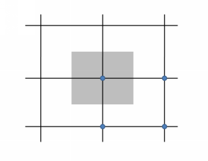
for the  field are available for the domain, a determination can be
made for the subdomains that surround every node (for example, the gray area
in Figure 4.27: A Control Volume Surrounding a Node) as to whether
field are available for the domain, a determination can be
made for the subdomains that surround every node (for example, the gray area
in Figure 4.27: A Control Volume Surrounding a Node) as to whether
 is above the threshold (which represents a "wet" node
condition) or below the threshold (which represents a “dry" node
condition). In this manner, the distribution of wet/dry nodes is known at
each time step.
is above the threshold (which represents a "wet" node
condition) or below the threshold (which represents a “dry" node
condition). In this manner, the distribution of wet/dry nodes is known at
each time step.
Because it is not possible to numerically integrate discontinuous data
without dissipation, the variation in the size of the wet domain is
generally lower than the net volume of fluid that entered the domain through
the inlets during the time step. To avoid translating this dissipation into
a volume loss, the Fluent Materials Processing workspace calibrates the elapsed time for a
successful time step based on the amount of fluid that entered the domain,
rather than simply equating it with  . Note that this calibration is only performed when the
flow rate of fluid entering the domain is nonzero; when no fluid enters (for
example, when no inlet is present), the elapsed time is set equal to the
initially defined value of the time step. For this reason, you should define
the initial time step conservatively.
. Note that this calibration is only performed when the
flow rate of fluid entering the domain is nonzero; when no fluid enters (for
example, when no inlet is present), the elapsed time is set equal to the
initially defined value of the time step. For this reason, you should define
the initial time step conservatively.
The following is a list of scenarios that can arise during the VOF
simulation, and the resulting impact on the evaluation of  and/or the simulation:
a positive net change in the number of wet nodes does not occur as a result of the time step, even though the inlet flow rate is not zero
This is an indication that Equation 4–3 has not been integrated over a period of time that is long enough to allow new nodes of the domain to reach the
 threshold, and so a larger time step must be
applied. In this case, the time step index is not incremented,
threshold, and so a larger time step must be
applied. In this case, the time step index is not incremented,
 is increased by 50%, and the calculations are run
again to compute the
is increased by 50%, and the calculations are run
again to compute the  field. This process can be repeated up to 10 times
for a particular time step, after which point the simulation is
terminated.
field. This process can be repeated up to 10 times
for a particular time step, after which point the simulation is
terminated. the ordinary flow calculation returns an error (for example, divergence is detected for a nonlinear problem)
In this case, the time step index is not incremented and the flow calculation is attempted again using a smaller value of
 . If no new wet nodes result and the calculation
still diverges, the algorithm will eventually stop.
. If no new wet nodes result and the calculation
still diverges, the algorithm will eventually stop. the calculations for a time step yields a positive net change in the number of wet nodes
This represents a successful outcome, and so the time step index is incremented. Having computed a new wet node flag vector (which yielded a new volume of fluid
 in the domain) as a result of the inlet flow rate
 , a new value for
  is calculated for the next time step as follows:
(4–4)
Here,
 is a parameter you can set to control the
Accuracy of the scheme, and can be specified in
the calculation activities panel (see Calculation Activities Properties). Recommended values of
is a parameter you can set to control the
Accuracy of the scheme, and can be specified in
the calculation activities panel (see Calculation Activities Properties). Recommended values of
 are on the order of 0.2–0.5. Note that an
extremely low value of
are on the order of 0.2–0.5. Note that an
extremely low value of  can reduce the time step to such a degree that no
new nodes become wet; consequently, the time step will be increased
as described previously, and you then run the risk of engaging in an
oscillatory "forward/backwards" marching scheme that calculates
several useless iterations without improved accuracy. An inherent
limitation of the VOF model is that it cannot process changes that
are smaller than the element size.
can reduce the time step to such a degree that no
new nodes become wet; consequently, the time step will be increased
as described previously, and you then run the risk of engaging in an
oscillatory "forward/backwards" marching scheme that calculates
several useless iterations without improved accuracy. An inherent
limitation of the VOF model is that it cannot process changes that
are smaller than the element size. Note that if the inlet flow rate
 for the time step was 0, Equation 4–4 is ignored and
  is set to the value you defined for the initial
time step.
is set to the value you defined for the initial
time step. the time step index is incremented beyond the maximum number
In this case, the simulation is terminated. The maximum number of time steps is used to stop simulations that have values for
 that are too low, and consequently run too long.
Because of the Courant-type limitation described previously, you
should expect a complete filling simulation to take several hundreds
time steps and set the maximum accordingly. By default, the maximum
number of time steps is set to 1000.
that are too low, and consequently run too long.
Because of the Courant-type limitation described previously, you
should expect a complete filling simulation to take several hundreds
time steps and set the maximum accordingly. By default, the maximum
number of time steps is set to 1000.  is set to a value lower than the minimum
 The simulation is terminated when
 falls below the minimum.
 the total outlet flow rate (integrated over all outlets) is 99% of the nonzero total inlet flow rate (that is, the flow in the cavity is established, but almost all of the fluid is leaving the domain)
By default, the Fluent Materials Processing workspace stops the simulation in such circumstances, even if the cavity has not been completely filled. In most cases, it is considered normal to terminate a VOF simulation when the flow exits the domain. The value of 99% is hardcoded in the Fluent Materials Processing workspace. This constraint is disabled for simulations in which there are no defined inlets, thereby allowing you to model the emptying of the cavity. You can also ignore this constraint by turning off the Stop Run When Cavity Full option in the calculation activities panel (see Calculation Activities Properties).
the fluid fraction variable
 exceeds the threshold value (for example, 0.5 when
tracking a single fluid) throughout the entire domain
exceeds the threshold value (for example, 0.5 when
tracking a single fluid) throughout the entire domain As stated previously, the fluid is determined to be present wherever
 is above the threshold value. Exceeding this value
throughout the domain indicates that the volume of fluid has
completely filled the cavity, and so the simulation is stopped by
default. You can ignore this constraint by retaining the default
value of
is above the threshold value. Exceeding this value
throughout the domain indicates that the volume of fluid has
completely filled the cavity, and so the simulation is stopped by
default. You can ignore this constraint by retaining the default
value of 0for the Filtering Threshold on Fluid Fraction entry in the calculation activities panel (see Calculation Activities Properties).
Foamed polymer is extruded to obtain very light insulation parts. Polyethylene with dissolved gas enters through the inlet section and flows through the converging section and the die land. Next, throughout the extrudate, the material is free to deform. The workspace does not consider the chemical aspects of the foaming, but only its physical aspect: as soon as the mixture leaves the die or at least when the pressure is low enough, the dissolved gas will expand and the bubbles will grow, leading to a severe diminution of the mixture density. The Arefmanesh model (described in Foaming Theory) is used for predicting this behavior.
The model of foaming should be considered only with extrusion involving free surfaces (see Modeling the Determination of Die Lip Shape (Inverse Extrusion) and Modeling the Prediction of Extrudate Shape (Direct Extrusion) for more information on how to define such cases), as the bubble growth is generally impaired in confined domains.
Figure 4.28: Extrusion of a Foamed Profile: Domains and Boundaries displays a sketch of a realistic model for the simulation of an extrusion flow involving foaming. From right to left, the mixture (grey) enters the die channel, flows through the channel, exits the die, and expands freely (extrudate in yellow).
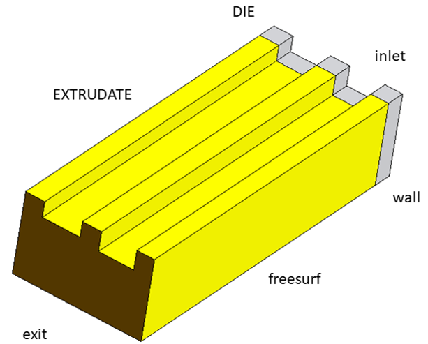
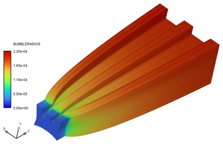
Figure 4.29: Extrusion of a Foamed Profile: Die Lip Shape Prediction and Bubble Radius Distribution displays the foamed profile and the bubble radius distribution for a case where the prediction of the die lip shape was requested.
The mandatory components are the following:
the geometry contains at least two zones (one for the flow within the die, one for the extrudate) and at least four boundaries (inlet, wall, free surface, exit),
appropriate material data,
boundary or operating conditions, such as flow rate, behaviour along the die wall, condition at the exit.
Rheological Models
Only the generalized Newtonian fluid models can be invoked, under both isothermal and thermal conditions. Default values are assigned to the several parameters, but it is always a good idea to check them. There are also material data files available in the Extrusion and Miscellaneous families in the Library of Materials.
Domains and Boundary Conditions
The calculation domain must contain at least two zones. One zone is needed for the calculation of the flow within the die, and another zone is needed for the calculation of the extrudate that deforms from the die exit until the exit of the calculation domain. A mesh deformation algorithm is applied on this latter zone. If a die lip prediction is requested, a mesh deformation must be also be defined on the die domain.
As can be seen in Figure 4.28: Extrusion of a Foamed Profile: Domains and Boundaries , the calculation domain is surrounded by at least four boundaries:
the inlet where a flow rate is usually assigned and where the workspace fixes the bubble radius,
the fixed die wall where slipping can be specified,
the outer border of the extrudate where free surface conditions are imposed, and
the exit of the calculation domain. On this latter border, a take-up force or velocity can be imposed, and a stress free condition is also possible.
Sometimes, additional boundaries are needed as this is typically the case when symmetry planes do exist and are taken into account.
Additional Modeling Features
There are actually limited possibilities for expanding the model used for calculating the foaming. Thermal effects can be considered, and require selecting appropriate material data such as thermal conductivity, heat capacity, as well as possible temperature dependence of material properties that also requires assigning thermal boundary conditions and specifying appropriate temperature initialization.
Note that the use of guiding devices with gravity effects also can play a visible role, and it is a good idea to define a conveyor belt or a roller conveyor, as is most likely present in the actual process.
Convergence Strategies
From the above description, a model for extrudate shape and or die lip prediction can involve several non-linearities originating from the geometry, the rheology, and the boundary conditions. To these non-linearities one can of course add the variable density and the bubble growth model. For facilitating the calculation, convergence strategies have been implemented and have been made available. Next to convergence strategy for free surfaces and moving interfaces that is highly recommended, you can also invoke convergence strategies for thermal flows, for rheology and slipping. Of course, the convergence strategy for foaming is mandatory. The required convergence strategies are not set by default, and you must select convergence strategies in accordance with the setup. Decoupling the computation of species may also help for the convergence.
Additional Information
There are additional resources for exploring this type of simulation:
For an example that demonstrates a foaming application, see Extrusion of a Foamed Profile.
The Arefmanesh model (References) is used for predicting the bubble growth occurring during the foaming process. The model assumes a purely viscous material, and that the time scale of gas diffusion is longer than that of bubble expansion. Hence, the diffusion of dissolved gas from the polymer into the bubble is neglected. The model is such that all physics is lumped in a single transport equation that dictates the bubble radius R:
 | (4–5) |
where pg is the gas pressure and
p is the matrix pressure. The parameter  plays the role of surface tension, as it slows down a bit of
the bubble growth. The quantity
plays the role of surface tension, as it slows down a bit of
the bubble growth. The quantity  is a macroscopic viscosity of the (dense) polymer matrix
around the bubble. The power index a may add some
non-linearities to the model. Eventually, parameter b is a
booster if the foaming is not as large as expected.
is a macroscopic viscosity of the (dense) polymer matrix
around the bubble. The power index a may add some
non-linearities to the model. Eventually, parameter b is a
booster if the foaming is not as large as expected.
A second aspect to consider is the way the density of the mixture depends on the number of bubbles and their size (assuming that the mass of the gas is negligible compared to the polymer matrix). The density ρ of the mixture is given by:
 | (4–6) |
where ρp is the density of the polymer matrix (without blowing agent, that is, with R equivalent to 0), and N is the number of cells per unit volume of gas/polymer mixture. Also, while foaming progresses, the macroscopic viscosity of our mixture decreases since the volume increase results only from gas expansion. Hence, with the bubble growth, the workspace assumes that the zero-shear viscosity of the mixture decreases in the same way as the density:
 | (4–7) |
where  is the zero-shear viscosity of the polymer matrix (without
blowing agent, that is, with R equivalent to 0).
is the zero-shear viscosity of the polymer matrix (without
blowing agent, that is, with R equivalent to 0).
The model does not necessarily predict an equilibrium bubble size: gas pressure decreases with increasing bubble radius but does not vanish. In actual cases, however, bubbles do not grow infinitely, since the polymer cools down and the extrudate shape freezes.
Many consumer products are made of two or more materials, for example to confer them specific visual, mechanical or chemical properties. The control of the interface between materials with different properties is therefore important for matching technological or market requirements. The workspace enables the simulation of coextrusion. Here the interface between adjacent materials is tracked by means of a transport variable, while velocity, pressure and possibly temperature are evaluated along the usual procedure. Such calculations can be performed inside a die, but may also involve the prediction of the extrudate shape.
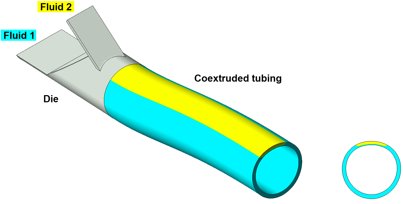
Figure 4.30: An Example of Coextrusion illustrates a coextrusion flow with a relatively simplified die for the production of coextruded tubing. From left to right, two materials, blue and yellow, enter the die through individual inlets, merge into the die before being subsequently dragged. In general, next to the prediction of the interface(s), such calculation provides useful output such as, but not limited to, velocity, pressure and temperature. Important components are the following:
the geometry with at least one zone and four boundaries (two inlets, wall, exit) when focussing on the internal coextrusion flow only, and at least two zones and five boundaries (two inlets, wall, free surface, exit) for the prediction of extrudate shape,
appropriate material data for at least two materials,
boundary or operating conditions, such as flow rates, behaviour along the die wall, condition at the exit.
Rheological Models
For setting up the calculation of coextrusion flow, all generalized Newtonian fluid models can be invoked, under both isothermal and thermal conditions. Default values are assigned to the several parameters, but it is always a good idea to check them. There are also material data files available in the Extrusion and Miscellaneous families in the Library of Materials.
Domains and Boundary Conditions
The calculation domain must contain at least two zones when the extrudate shape is predicted, one for the flow within the channel, and one for the extrudate. A mesh deformation algorithm is applied on this latter zone, that may significantly deform due to velocity rearrangement as well as to the take-up velocity or force.
The calculation domain shown in Figure 4.30: An Example of Coextrusion is surrounded by seven boundaries:
two inlets where flow rates are assigned,
the fixed inner and outer channel walls where slipping can be specified,
the inner and outer free surfaces of the coextruded tubing, and
the exit of the calculation domain.
On this latter border, a take-up force or velocity can be imposed. Sometimes, additional boundaries are needed: for example, when symmetry planes do exist and are taken into account into the model.
Additional Modeling Features
When the extrudate prediction is involved, the present coextrusion model can be expanded by adding a few more features. Thermal effects, including conjugated heat transfer with the solid die, can be considered. This requires specifying appropriate material data such as thermal conductivity, heat capacity, as well as possible temperature dependence of material properties, it also requires assigning thermal boundary conditions and specifying appropriate temperature initialization.
Specific features can be added for the extrudate, such as take-up force or velocity, free jet stabilization for small profiles, and conveyor belt or rollers for heavy profiles.
The coextrusion model can also be used for die lip shape determination, however, it is important to remember that the extrudate shape is dictated while the interface between fluid layers cannot be controlled.
Convergence Strategies
From the above description, the primary source of non-linearity in the setup for the calculation of a coextrusion flow originates from the interface prediction. For facilitating the calculation, convergence strategies have been implemented and made available, and you must select them in accordance with the setup. Next to convergence strategy for multiple materials that is often recommended here, you can also invoke convergence strategies for viscosity and slipping, free surfaces and/or for thermal flows.
Additional Information
There are additional resources for exploring this type of simulation:
To use a template for the calculation of coextrusion flow, see Using the Extrusion Template.
For a tutorial that demonstrates coextrusion, see Multiple Material Coextruded Tubing.
An important component of the fiber spinning or fiber drawing process occurs where a molten polymer filament is stretched at a high velocity in order to produce a fiber of very small transverse dimensions. Typical transverse dimensions of synthetic fibers can be of the order of 10 µm; typical take-up velocities are often of the order of 100 m/s at some distance from the spinneret, they are however significantly smaller in the vicinity of the spinneret.
To some extent, modeling fiber spinning process does not significantly differ from profile extrusion. However, dimensions are much smaller, so that gravity effects can be neglected, while heat transfer as well as rheology may play a visible role. Without unnecessarily loading a model, stretching, cooling and strain hardening are three major effects that can be considered, probably with decreasing priorities
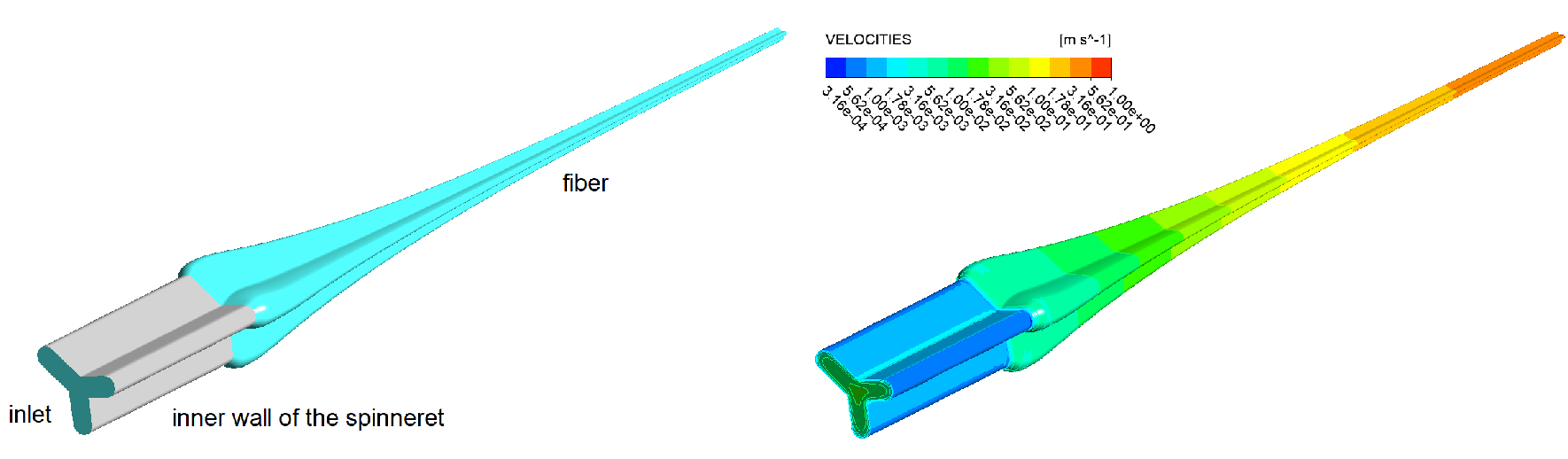
Figure 4.31: An Example of Fiber Spinning illustrates a simple model for the spinning simulation of a non-symmetric tri-lobal fiber (left), together with the distribution of the velocity magnitude at the inlet, on the inner wall of the spinneret and the fiber free surface (right), presently up to a downstream length of 20 mm.
From left to right, the melt (light blue) enters a channel of the spinneret (grey), flows through a channel of the spinneret, exits the channel, and is subsequently pulled at a high take-up force or velocity. The following components are needed:
the geometry contains at least two zones (for the flow within the channel, and for the fiber) and at least four boundaries (inlet, wall, free surface, exit),
appropriate material data,
boundary or operating conditions, such as flow rate, behavior along the die wall, take-up force or velocity.
Rheological Models
For setting up the simulation of fiber spinning, all generalized Newtonian fluid models, differential viscoelastic models, as well as the simplified viscoelastic model are available, under isothermal and thermal conditions. However, since elongation of the fiber is presumably more important than material shear-thinning in the channel, you should consider a model that exhibits some amount of strain hardening, or at least no thinning in extension.
Domains and Boundary Conditions
The calculation domain must contain at least two zones, one for the flow within the channel and one for the fiber. A mesh deformation algorithm is applied on this latter zone, which may significantly deform due to the take-up velocity or force.
As shown in Figure 4.31: An Example of Fiber Spinning, the calculation domain is surrounded by at least four boundaries:
the inlet where a flow rate is usually assigned,
the fixed channel wall where slipping can be specified,
the free surface of the fiber, and
the exit of the calculation domain.
On this latter border, a take-up force or velocity is imposed. Sometimes, additional boundaries are needed: for example, when symmetry planes do exist and are taken into account into the model.
Additional Modeling Features
The present simple model for fiber spinning can be expanded. Primarily, thermal effects can be considered that require additional material data as well as assigning thermal boundary conditions and specifying temperature initialization. Conjugated heat transfer with the die is also possible.
Specific features can be selected for the fiber. If moderate draw-down effects are expected, it can be useful to invoke the free jet stabilization when the profile lacks symmetry. For high draw-down effects, stabilization is often naturally recovered.
Convergence Strategies
A model for fiber spinning can involve several non-linearities originating from the geometry, the rheology, and the boundary conditions. For facilitating the calculation, convergence strategies can be activated. Next to convergence strategy for free surfaces and moving interfaces which is often recommended, you can also activate convergence strategies for thermal flows, for rheology and slipping, as well as for the take-up force or velocity.
Related Notes
Avoid using a model intrinsically characterized by strain-thinning behavior. The simplified viscoelastic model has no real added value in fiber spinning.
The assigned take-up velocity should never vanish.
Very thin thermal boundary layers can develop along the fiber surface, due to the combination of small transverse dimensions and large velocities.
Additional Information
There are additional resources for exploring this type of simulation:
To use a template for the prediction of extrudate shape, see Using the Extrusion Template.
For an example that demonstrates the simulation of fiber spinning of a viscoelastic fluid, see Spinning Simulation of a Non-Symmetric Trilobal Viscoelastic Fiber.
When modeling a semi-transparent medium, it can be important to account for radiation internal to the material. This is especially true when very high temperatures are involved, as can be the case in glass processing. Fluent Materials Processing allows you to calculate internal radiation using the P-1 radiation approximation model.
The P-1 model can be solved for fixed or moving geometry, with the mesh encapsulating the radiative domain. The P-1 model involves the calculation of a new variable, namely the incident radiation. Therefore, it should achieve more accurate results than those obtained by using the Rosseland correction at the boundary combined with a third order polynomial expression for the thermal conductivity, and is also computationally more expensive.
As shown below, there is an obvious connection between radiation and
temperature. However, the radiation is not affected by the motion of the
material since the incident radiation, as an electromagnetic signal, propagates
at the speed of light in the material. The model involves the calculation of the
heat equation for the temperature and a conduction equation for the incident
radiation. Both equations are coupled through a source term and through boundary
conditions.  and
and  respectively denote the temperature and the incident
radiation. These variables obey the following equations:
respectively denote the temperature and the incident
radiation. These variables obey the following equations:


Several material parameters are involved in the above equations. Next to
density  , the heat capacity
  and the thermal conductivity
  , is the incident radiation diffusion coefficient
 , the absorption coefficient
  , the refractive index
  , and the Stefan-Boltzmann constant
  (5.670374 10-8
W/m2/K4).
(5.670374 10-8
W/m2/K4).  is a source term which accounts for the viscous heating. The
absorption coefficient
is a source term which accounts for the viscous heating. The
absorption coefficient  (or the reciprocal of the optical depth) characterizes the
opacity (or the transparency) of the material, while the refractive index
(or the reciprocal of the optical depth) characterizes the
opacity (or the transparency) of the material, while the refractive index
 is the ratio between the speed of light in a vacuum and that
through a semi-transparent medium and is always greater than 1. In general, the
diffusion coefficient
is the ratio between the speed of light in a vacuum and that
through a semi-transparent medium and is always greater than 1. In general, the
diffusion coefficient  for the incident radiation is given by:

As shown above, it is dependent on the absorption coefficient  , the scattering coefficient
  and the linear anisotropic phase function coefficient
 . The scattering coefficient is a property that describes the
capability of particles to scatter photons. The linear anisotropic phase
function coefficient ranges from -1 to 1 and indicates whether radiant energy is
dominantly scattered forward (
. The scattering coefficient is a property that describes the
capability of particles to scatter photons. The linear anisotropic phase
function coefficient ranges from -1 to 1 and indicates whether radiant energy is
dominantly scattered forward ( > 0) or backward (
 < 0), a zero value defines isotropic scattering. When
scattering is discarded, i.e., when
< 0), a zero value defines isotropic scattering. When
scattering is discarded, i.e., when  = 0, then
  .
.
The above advection/diffusion equations are subjected to boundary conditions.
When symmetry condition is applied for the flow, it is also applied for the
temperature and for the incident radiation as well. In the other circumstances,
the selected boundary condition for the incident radiation is independent from that of the temperature: the temperature
boundary conditions are then of the usual type (symmetry, insulated, heat flux,
convection, temperature imposed), while either insulated or opaque boundary
condition can be selected for the incident radiation. Opaque boundary condition
obeys the following equation:

where  is the emissivity coefficient of the boundary surface, which
ranges from 0 (mirror) to 1 (black body). When the opaque boundary condition is
selected, the emissivity coefficient
is the emissivity coefficient of the boundary surface, which
ranges from 0 (mirror) to 1 (black body). When the opaque boundary condition is
selected, the emissivity coefficient  must be specified.
To set up a thermal calculation with radiation, you must perform the following:
A thermal flow problem must be defined.
Specify the additional material properties for radiation.
Activate the calculation for radiation.
Assign boundary conditions for the radiation.
Activate the convergence strategy for the radiation.
You can specify the Radiation Properties within the Properties - fluid panel.
![]() Setup →
Materials → fluid
Setup →
Materials → fluid
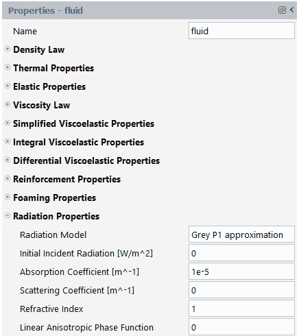
The default values of the parameters correspond to a nearly perfectly
transparent material with a very low absorption coefficient, (or equivalent to a long optical depth  ), no scattering and a unit refractive index
. You can also specify a value for the Initial
Incident Radiation which will only be used for initializing the
corresponding field, facilitating convergence. A reasonable order of
magnitude for the initial Initial Incident Radiation
can be
), no scattering and a unit refractive index
. You can also specify a value for the Initial
Incident Radiation which will only be used for initializing the
corresponding field, facilitating convergence. A reasonable order of
magnitude for the initial Initial Incident Radiation
can be  .
.
Activate radiation in the Properties - fluid-zone panel.
![]() Setup → Cell
Zones → fluid-zone
Setup → Cell
Zones → fluid-zone
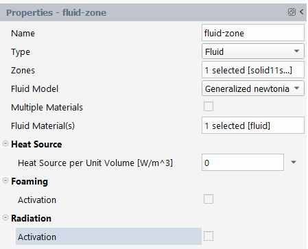
Once radiation is activated, you can optionally specify whether the incident radiation field will be calculated (default selection) or frozen to a specified value.
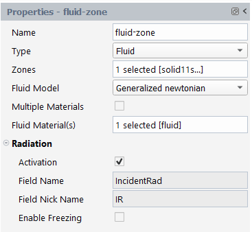
In the Properties panels, under Boundary Conditions, you must select the boundary conditions for the incident radiation in addition to the flow and temperature boundary requirements.
![]() Setup → Boundary
Conditions → wall
Setup → Boundary
Conditions → wall
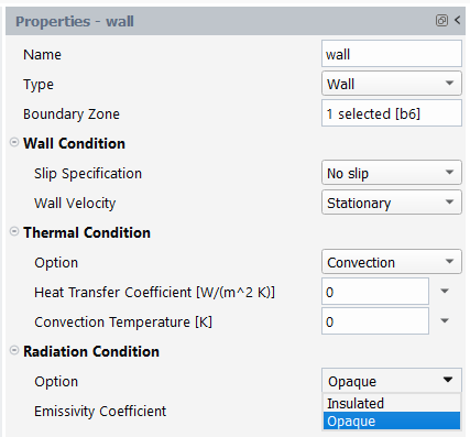
You can choose whether the radiation condition is or . In the latter case, the Emissivity Coefficient at the boundary surface must be given.