

This section contains a listing of the contents for the various property panels available in the Fluent Materials Processing workspace.
General property settings are used to define the overall simulation. Here, you can view and adjust any geometry, mesh, or calculation settings, as well as assorted physics options.
Controls
- Mesh file
Indicates the location and name of the mesh file. For more information, see Meshes in the Polyflow documentation.
- Mesh length unit
Indicates the unit of length used in the mesh file. For more information, see Units in the Polyflow documentation.
- Mesh Format
Indicates the format of the mesh file
- Box Size
Describes the dimensions of the mesh.
- Geometry Type
Indicates the dimensionality of the geometry to be represented by the mesh file. If the mesh is a 2D plane, the simulation may be planar (Vz equal to 0), channel (Vz not equal to 0), axisymmetric (Y axis being the axis of symmetry + Vw = 0), swirling (axisymmetric, with the Y axis being the axis of symmetry + Vw not equal to 0) and film (planar + thickness(es)). Note: Vw is the rotation velocity around the Y axis.
- Calculation Type
Indicates the specific type of calculation to be performed. Calculations can be Steady, Continuation, Transient, or Volume of Fluid when you want to perform a transient simulation of a filling process.
- Task name
Specify a name for the task.
- Duration
For a transient or volume of fluid calculation, specify the overall length of time interval.
- Include thermal effects
Enable this option if you want to model fluid flow in which temperature plays a role.
- Include inertia effects
Enable this option if you want to model fluid flow in which inertia plays a role. For blow molding simulations, inertia effects are always included.
- Include viscous dissipation effects
Enable this option if you want to model the heat generated by internal forces and friction along slipping walls.
- Include gravity effects
Enable this option if you want to model fluid flow in which gravity plays a role. When selected, for the Gravity definition, enter the X, Y, and Z components of the gravitational acceleration.
- Gx
Specify the value of the x-component of the gravitational acceleration. Using the drop-down menu, you can enter a constant value, or a valid expression.
- Gy
Specify the value of the y-component of the gravitational acceleration. Using the drop-down menu, you can enter a constant value, or a valid expression.
- Gz
Specify the value of the z-component of the gravitational acceleration. Using the drop-down menu, you can enter a constant value, or a valid expression.
Material property settings for your simulation.
All that is required here is to specify a value for the density for the material used in the simulation.
- Density
Specify the density of the material. Using the drop-down menu, you can enter a constant value, or a valid expression.
This section contains settings for thermal-related properties such as thermal expansion, thermal conductivity and heat capacity. For additional information, see Basic Equations in the Polyflow User's Guide.
Thermal Expansion
Thermal expansion can be equated to the Boussinesq approximation that can be used instead of a constant density. For additional information, see Boussinesq Approximation for Density in Nonisothermal Flows in the Polyflow User's Guide.
- Coefficient of thermal expansion
Coefficient of thermal expansion used within the context of the Boussinesq approximation, that is, the effect is applied only on the volume forces (gravity)
- Reference temperature
Within the context of the Boussinesq approximation for the thermal expansion: temperature at which thermal expansion vanishes, that is, at which the density is equal to the specified Density value.
Thermal Conductivity
- K
Select a constant thermal conductivity (K) or a third-order, temperature-dependent, polynomial expression.
- A
When the thermal conductivity law is set to Constant, specify a constant value for the thermal conductivity, or a valid expression. Otherwise, when the law is set to Polynomial, specify the primary coefficient of the thermal conductivity polynomial expression; it may not vanish.
- B
The coefficient of the linear term in the temperature-dependent thermal conductivity polynomial expression.
- C
The coefficient of the quadratic term in the temperature-dependent thermal conductivity polynomial expression.
- D
The coefficient of the cubic term in the temperature-dependent thermal conductivity polynomial expression.
- Reference temperature
Specify the temperature at which the thermal conductivity is constant and is equal to the primary coefficient A.
Heat Capacity
- Cp
Select a constant heat capacity per unit mass or a third-order, temperature-dependent, polynomial expression.
- A
When the heat capacity per unit mass law is set to Constant, specify a constant value for the heat capacity per unit mass, or a valid expression. Otherwise, when the law is set to Polynomial, specify the primary coefficient of the polynomial expression for the heat capacity per unit mass.
- B
The coefficient of the linear term in the temperature-dependent heat capacity per unit mass polynomial expression.
- C
The coefficient of the quadratic term in the temperature-dependent heat capacity per unit mass polynomial expression.
- D
The coefficient of the cubic term in the temperature-dependent heat capacity per unit mass polynomial expression.
- Reference temperature
Specify the temperature at which the heat capacity per unit mass is constant and is equal to the primary coefficient A.
This section contains descriptions of a material's elastic properties. For additional information, see Theory in the Polyflow User's Guide.
Young Modulus
- E
Specify a value for E, the Young modulus.
Poisson Coefficient
- Mu
Specify a value for mu, for the Poisson coefficient.
Lineic Dilatation Coefficient
- Alpha
For linear thermo-elasticity, specify a value for alpha, the lineic dilitation coefficient.
- Reference temperature
For linear thermo-elasticity, specify the temperature at which lineic dilatation vanishes.
This section holds details pertaining to a material's viscosity definition.
- Shear-rate dependency model
Specify the shear-rate dependence model.
- Temperature dependency model
Choose the model for the temperature dependence.
Allows you to specify a constant value for the viscosity. For additional information, see Constant in the Polyflow User's Guide.
- Viscosity
Specify a value for the viscosity. Using the drop-down menu, you can enter a constant value, or a valid expression.
Allows you to specify the properties of the Power Law viscosity model. For additional information, see Power Law in the Polyflow User's Guide.
- Consistency factor
The viscosity at shear-rate equal to the inverse of the Time Constant.
- Time constant
The inverse of the shear-rate at which the viscosity is equal to the Consistency Factor.
- Power law index
An index ranging between 0 and 1; it quantifies the rate of shear thinning. On a log-log diagram, the index corresponds to the slope of shear stress curve versus shear rate. A value of 1 corresponds to a constant viscosity Newtonian fluid, while values lower than 1 indicate shear thinning.
Allows you to specify the properties of the Bird-Carreau Law viscosity model. For additional information, see Bird-Carreau Law in the Polyflow User's Guide.
- Zero shear viscosity
The viscosity at zero shear-rate.
- Time constant
Natural time. That is, inverse of the shear rate at which the fluid changes from a Newtonian to a power-law behavior.
- Power law index
An index ranging between 0 and 1; it quantifies the rate of shear thinning that occurs beyond a shear rate equal to the inverse of the time constant. A value of 1 corresponds to a constant viscosity Newtonian fluid, while the amount of shear thinning increases when the power index decreases down to 0.
- Infinite shear viscosity
The asymptotic value of the shear viscosity at very high shear rate.
Allows you to specify the properties of the Carreau-Yasuda Law viscosity model. For additional information, see Carreau-Yasuda Law in the Polyflow User's Guide.
- Zero shear viscosity
Viscosity at zero shear-rate.
- Time constant
Natural time. That is, inverse of the shear rate at which the fluid changes from Newtonian to power-law behavior.
- Power law index
An index ranging between 0 and 1; it quantifies the rate of shear thinning that occurs beyond a shear rate equal to the inverse of the time constant. A value of 1 corresponds to a constant viscosity Newtonian fluid, while the amount of shear thinning increases when the power index decreases down to 0.
- Infinite shear viscosity
The asymptotic value of the shear viscosity at very high shear rate.
- Plateau index
Parameter that controls the rate of transition from the Newtonian viscosity plateau at low shear rate to the shear thinning behavior. A value between 0 and 1 leads to a rather smooth transition, while higher values lead to a sharp transition.
Allows you to specify the properties of the Bingham Law viscosity model. For additional information, see Bingham Law in the Polyflow User's Guide.
- Plastic viscosity
On a linear diagram, the plastic viscosity indicates the slope of the shear stress curve versus shear rate beyond the yield stress threshold. It also corresponds to the asymptotic value of the shear viscosity at very high shear rate.
- Yield stress threshold
Ideally, the yield stress threshold is the minimum amount of stress that is needed to apply a deformation to the material. In the CFD context, it corresponds to the stress level below which very little deformation is exhibited by the fluid.
- Critical shear rate
The critical shear rate controls the rate of transition between the no-flow behavior when the local stress level is less than the yield stress threshold and the fluid response when the stress is large enough. The rate of transition increases when the critical shear rate decreases.
Allows you to specify the properties of the Modified Bingham Law viscosity model. For additional information, see Modified Bingham Law in the Polyflow User's Guide.
- Plastic viscosity
On a linear diagram, the plastic viscosity indicates the slope of the shear stress curve versus shear rate beyond the yield stress threshold. It also corresponds to the asymptotic value of the shear viscosity at very high shear rate.
- Yield stress threshold
Ideally, the yield stress threshold is the minimum amount of stress that is needed to apply a deformation to the material. In the CFD context, it corresponds to the stress level below which very little deformation is exhibited by the fluid.
- Critical shear rate
The critical shear rate controls the rate of transition between the no-flow behavior when the local stress level is less than the yield stress threshold and the fluid response when the stress is large enough. The rate of transition increases when the critical shear rate decreases.
Allows you to specify the properties of the Herschel-Bulkley Law viscosity model. For additional information, see Herschel-Bulkley Law in the Polyflow User's Guide.
- Yield stress threshold
Ideally, the yield stress threshold is the minimum amount of stress that is needed to apply a deformation to the material. In the CFD context, it corresponds to the stress level below which very little deformation is exhibited by the fluid.
- Consistency factor
On a linear diagram, the consistency factor indicates the shear stress growth versus shear rate beyond the yield stress threshold.
- Power law index
On a linear diagram, the power law index indicates the change of slope of the shear stress growth versus shear rate beyond the yield stress threshold. The rate of shear thinning increases when the index decreases down to 0.
- Critical shear rate
The critical shear rate controls the rate of transition between the no-flow behavior when the local stress level is less than the yield stress threshold and the fluid response when the stress is large enough. The rate of transition increases when the critical shear rate decreases.
Allows you to specify the properties of the Modified Herschel-Bulkley Law viscosity model. For additional information, see Modified Herschel-Bulkley Law in the Polyflow User's Guide.
- Yield stress threshold
Ideally, the yield stress threshold is the minimum amount of stress that is needed to apply a deformation to the material. In the CFD context, it corresponds to the stress level below which very little deformation is exhibited by the fluid.
- Consistency factor
On a linear diagram, the consistency factor indicates the shear stress growth versus shear rate beyond the yield stress threshold.
- Power law index
On a linear diagram, the power law index indicates the change of slope of the shear stress growth versus shear rate beyond the yield stress threshold. The rate of shear thinning increases when the index decreases down to 0.
- Critical shear rate
The critical shear rate controls the rate of transition between the no-flow behavior when the local stress level is less than the yield stress threshold and the fluid response when the stress is large enough. The rate of transition increases when the critical shear rate decreases.
Allows you to specify the properties of the Cross Law viscosity model. For additional information, see Cross Law in the Polyflow User's Guide.
- Zero shear viscosity
Viscosity at zero shear-rate.
- Time constant
Natural time. That is, inverse of the shear rate at which the fluid changes from a Newtonian to a power-law behavior.
- Cross law index
Index that controls the rate at which the viscosity decreases with increasing shear-rate. A value of 0 corresponds to a Newtonian fluid (no shear thinning), a value of 1 corresponds to a viscosity that decreases rapidly (important shear thinning)
Allows you to specify the properties of the Modified Cross Law viscosity model. For additional information, see Modified Cross Law in the Polyflow User's Guide.
- Zero shear viscosity
The viscosity at zero shear-rate.
- Time constant
Natural time. That is, inverse of the shear rate at which the fluid changes from a Newtonian to a power-law behavior.
- Cross law index
Index that controls the rate at which the viscosity decreases with increasing shear-rate. A value of 0 corresponds to a Newtonian fluid (no shear thinning), a value of 1 corresponds to a viscosity that decreases rapidly (important shear thinning)
Allows you to specify the properties of the Arrhenius Law temperature dependency viscosity model. For additional information, see Arrhenius Law in the Polyflow User's Guide.
- Activation energy
Specify the ratio of the activation energy to the thermodynamic constant.
- Reference temperature
Specify the temperature at which the function describing the temperature dependence is one. It often corresponds to the temperature of the master curve.
- Shift
Dictates how the viscosity will change with temperature: a vertical shift means that the viscosity curve is simply shifted downwards in a viscosity/shear-rate diagram when temperature increases, a vertical and horizontal shift means that the viscosity curve is shifted downwards and to the right when temperature increases.
Allows you to specify the properties of the Arrhenius Approximate Law temperature dependency viscosity model. For additional information, see Approximate Arrhenius Law in the Polyflow User's Guide.
- Activation energy
Specify the ratio of the activation energy to the thermodynamic constant.
- Reference temperature
Specify the temperature at which the function describing the temperature dependence is one. It often corresponds to the temperature of the master curve.
- Shift
Dictates how the viscosity will change with temperature: a vertical shift means that the viscosity curve is simply shifted downwards in a viscosity/shear-rate diagram when temperature increases, a vertical and horizontal shift means that the viscosity curve is shifted downwards and to the right when temperature increases.
Allows you to specify the properties of the Fulcher temperature dependency viscosity model. For additional information, see Fulcher Law in the Polyflow User's Guide.
- F1
Coefficient that can be used for applying an overall vertical shift of the viscosity curve versus temperature. It is redundant with the zero shear viscosity.
- F2
Coefficient that affects the slope of the decay of the viscosity curve with increasing temperature.
- F3
Temperature corresponding to the vertical asymptote of the viscosity curve versus temperature. In other words, it is the temperature at which the model would predict an infinite viscosity, suggesting fusion or solidification.
Allows you to specify the properties of the WLF temperature dependency viscosity model. For additional information, see WLF Law in the Polyflow User's Guide.
- C1
Empirical constant of the Williams-Landel-Ferry (WLF) law, which dictates the intensity of the temperature dependence.
- C2
Empirical constant of the Williams-Landel-Ferry (WLF) law, which dictates the intensity of the temperature dependence.
- Reference temperature
A temperature parameter which is sometimes related to the glass transition temperature of the material.
- Reference temperature difference
A temperature shift applied when considering another reference temperature. (For example, when considering another temperature for the master curve)
- Shift
Dictates how the viscosity will change with temperature: a vertical shift means that the viscosity curve is simply shifted downwards in a viscosity/shear-rate diagram when temperature increases, a vertical and horizontal shift means that the viscosity curve is shifted downwards and to the right.
This section holds details pertaining to a material's properties when using the Simplified Viscoelastic model. For additional information, see Simplified Viscoelastic Model in the Polyflow User's Guide.
- Weighting Coefficient
At the first approximation, it controls the swelling intensity versus flow rate. Use swelling-based experimental data to fine-tune the values for this property.
This section holds details pertaining to a material's viscosity definition when using the Simplified Viscoelastic model.
- Shear-rate dependency model
Specify the shear-rate dependence model.
Options include:
Allows you to specify a constant value for the viscosity when using the Simplified Viscoelastic model.
- Viscosity
Specify a value for the viscosity. Using the drop-down menu, you can enter a constant value, or a valid expression.
Allows you to specify a Power shear law when using the simplified viscoelastic model.
- Consistency factor
The viscosity at shear-rate equal to the inverse of the Time Constant.
- Time constant
The inverse of the shear-rate at which the viscosity is equal to the Consistency Factor.
- Power law index
An index ranging between 0 and 1; it quantifies the rate of shear thinning. On a log-log diagram, the index corresponds to the slope of shear stress curve versus shear rate. A value of 1 corresponds to a constant viscosity Newtonian fluid, while values lower than 1 indicate shear thinning.
Allows you to specify a Bird-Carreau shear law when using the simplified viscoelastic model.
- Zero first normal viscosity
The viscosity at zero shear-rate.
- Time constant
Natural time. That is, inverse of the shear rate at which the fluid changes from a Newtonian to a power-law behavior.
- Power law index
An index ranging between 0 and 1; it quantifies the rate of shear thinning that occurs beyond a shear rate equal to the inverse of the time constant. A value of 1 corresponds to a constant viscosity Newtonian fluid, while the amount of shear thinning increases when the power index decreases down to 0.
- Infinite first normal viscosity
The asymptotic value of the shear viscosity at very high shear rate.
Allows you to specify a Carreau-Yasuda shear law when using the simplified viscoelastic model.
- Zero first normal viscosity
Viscosity at zero shear-rate.
- Time constant
Natural time. That is, inverse of the shear rate at which the fluid changes from Newtonian to power-law behavior.
- Power law index
An index ranging between 0 and 1; it quantifies the rate of shear thinning that occurs beyond a shear rate equal to the inverse of the time constant. A value of 1 corresponds to a constant viscosity Newtonian fluid, while the amount of shear thinning increases when the power index decreases down to 0.
- Infinite first normal viscosity
The asymptotic value of the shear viscosity at very high shear rate.
- Plateau index
Parameter that controls the rate of transition from the Newtonian viscosity plateau at low shear rate to the shear thinning behavior. A value between 0 and 1 leads to a rather smooth transition, while higher values lead to a sharp transition.
Allows you to specify a Cross shear law when using the simplified viscoelastic model.
- Zero first normal viscosity
Viscosity at zero shear-rate.
- Time constant
Natural time. That is, inverse of the shear rate at which the fluid changes from a Newtonian to a power-law behavior.
- Cross law index
Index that controls the rate at which the viscosity decreases with increasing shear-rate. A value of 0 corresponds to a Newtonian fluid (no shear thinning), a value of 1 corresponds to a viscosity that decreases rapidly (important shear thinning)
Allows you to specify a modified Cross shear law when using the simplified viscoelastic model.
- Zero first normal viscosity
The viscosity at zero shear-rate.
- Time constant
Natural time. That is, inverse of the shear rate at which the fluid changes from a Newtonian to a power-law behavior.
- Cross law index
Index that controls the rate at which the viscosity decreases with increasing shear-rate. A value of 0 corresponds to a Newtonian fluid (no shear thinning), a value of 1 corresponds to a viscosity that decreases rapidly (important shear thinning)
Allows you to specify the first normal viscosity when using the simplified viscoelastic model.
- Shear-rate dependency model
Specify the law for the dependence of the first normal viscosity with respect to the pseudo shear-rate.
You can choose to use the same law as shear viscosity, or you can select from the following:
Allows you to specify a constant first normal viscosity law when using the simplified viscoelastic model.
- Viscosity
The normal viscosity at any pseudo shear rate.
Allows you to specify a Power first normal viscosity law when using the simplified viscoelastic model.
- Consistency factor
The viscosity at pseudo shear-rate equal to the inverse of the Time Constant.
- Time constant
The inverse of the pseudo shear-rate at which the normal viscosity is equal to the Consistency Factor.
- Power law index
An index ranging between 0 and 1; it quantifies the rate of shear thinning. On a log-log diagram, the index corresponds to the slope of shear stress curve versus pseudo shear rate. A value of 1 corresponds to a constant normal viscosity Newtonian fluid, while values lower than 1 indicate shear thinning.
Allows you to specify a Bird-Carreau first normal viscosity law when using the simplified viscoelastic model.
- Zero first normal viscosity
The normal viscosity at zero pseudo shear-rate.
- Time constant
Natural time. That is, inverse of the pseudo shear rate at which the fluid changes from a Newtonian to a power-law behavior.
- Power law index
An index ranging between 0 and 1; it quantifies the rate of shear thinning that occurs beyond a pseudo shear rate equal to the inverse of the time constant. A value of 1 corresponds to a constant normal viscosity Newtonian fluid, while the amount of shear thinning increases when the power index decreases down to 0.
- Infinite first normal viscosity
The asymptotic value of the normal viscosity at very high pseudo shear rate.
Allows you to specify a Carreau-Yasuda first normal viscosity law when using the simplified viscoelastic model.
- Zero first normal viscosity
The normal viscosity at zero pseudo shear-rate.
- Time constant
Natural time. That is, inverse of the pseudo shear rate at which the fluid changes from Newtonian to power-law behavior.
- Power law index
An index ranging between 0 and 1; it quantifies the rate of shear thinning that occurs beyond a pseudo shear rate equal to the inverse of the time constant. A value of 1 corresponds to a constant normal viscosity Newtonian fluid, while the amount of shear thinning increases when the power index decreases down to 0.
- Infinite first normal viscosity
The asymptotic value of the normal viscosity at very high pseudo shear rate.
- Plateau index
Parameter that controls the rate of transition from the Newtonian normal viscosity plateau at low pseudo shear rate to the shear thinning behavior. A value between 0 and 1 leads to a rather smooth transition, while higher values lead to a sharp transition.
Allows you to specify a Cross first normal viscosity law when using the simplified viscoelastic model.
- Zero first normal viscosity
The normal viscosity at zero pseudo shear-rate.
- Time constant
Natural time. That is, inverse of the pseudo shear rate at which the fluid changes from a Newtonian to a power-law behavior.
- Cross law index
Index that controls the rate at which the normal viscosity decreases with increasing pseudo shear-rate. A value of 0 corresponds to a Newtonian fluid (no shear thinning), a value of 1 corresponds to a normal viscosity that decreases rapidly (important shear thinning)
Allows you to specify a modified Cross first normal viscosity law when using the simplified viscoelastic model.
- Zero first normal viscosity
The viscosity at zero shear-rate.
- Time constant
Natural time. That is, inverse of the pseudo shear rate at which the fluid changes from a Newtonian to a power-law behavior.
- Cross law index
Index that controls the rate at which the normal viscosity decreases with increasing pseudo shear-rate. A value of 0 corresponds to a Newtonian fluid (no shear thinning), a value of 1 corresponds to a viscosity that decreases rapidly (important shear thinning)
Allows you to specify the relaxation time law when using the simplified viscoelastic model.
- Shear-rate dependency model
Specify the model for the shear rate dependence.
Options include:
Allows you to specify a constant relaxation time law when using the simplified viscoelastic model.
- Facr
It affects the speed at which the pseudo shear rate changes subsequent to a change in the local shear rate. Additionally, in first approximation, it affects the speed at which the extrudate swelling develops. Use swelling-based experimental data to fine-tune the values for this property.
Allows you to specify a Power relaxation time law when using the simplified viscoelastic model.
- Facr
The relaxation time at shear-rate equal to the inverse of the Time Constant.
- Tnatr
The inverse of the shear-rate at which the relaxation time is equal to the Consistency Factor.
- Expor
An index that controls the rate at which the relaxation time decreases with increasing shear-rate. A value of 1 corresponds to a constant relaxation time, a low value corresponds to a relaxation time that decreases rapidly.
Allows you to specify a Bird-Carreau relaxation time law when using the simplified viscoelastic model.
- Facr
The relaxation time at zero shear-rate.
- Tnatr
Natural time. That is, inverse of the shear-rate at which the relaxation time starts to decrease with an increasing shear-rate.
- Expor
An index that controls the rate at which the relaxation time decreases with increasing shear-rate. A value of 1 corresponds to a constant relaxation time, a low value corresponds to a relaxation time that decreases rapidly.
Allows you to specify the material's thermal dependency properties when using the Simplified Viscoelastic model.
- Temperature dependency model
Choose the model for the temperature dependence.
- Thermal dependency applied on relaxation time
By default, the temperature dependence is applied only on the viscosity and first normal viscosity laws. Optionally it can also be applied on the relaxation time.
Allows you to specify the properties of the Arrhenius Law temperature dependency viscosity model when using the Simplified Viscoelastic model.
- Activation energy
Specify the ratio of the activation energy to the thermodynamic constant.
- Reference temperature
Specify the temperature at which the function describing the temperature dependence is one. It often corresponds to the temperature of the master curve.
- Shift
Dictates how the viscosity will change with temperature: a vertical shift means that the viscosity curve is simply shifted downwards in a viscosity/shear-rate diagram when temperature increases, a vertical and horizontal shift means that the viscosity curve is shifted downwards and to the right when temperature increases.
Allows you to specify the properties of the Arrhenius Approximate Law temperature dependency viscosity model when using the Simplified Viscoelastic model.
- Activation energy
Specify the ratio of the activation energy to the thermodynamic constant.
- Reference temperature
Specify the temperature at which the function describing the temperature dependence is one. It often corresponds to the temperature of the master curve.
- Shift
Dictates how the viscosity will change with temperature: a vertical shift means that the viscosity curve is simply shifted downwards in a viscosity/shear-rate diagram when temperature increases, a vertical and horizontal shift means that the viscosity curve is shifted downwards and to the right when temperature increases.
Allows you to specify the properties of the WLF temperature dependency viscosity model when using the Simplified Viscoelastic model.
- C1
Empirical constant of the Williams-Landel-Ferry (WLF) law, which dictates the intensity of the temperature dependence.
- C2
Empirical constant of the Williams-Landel-Ferry (WLF) law, which dictates the intensity of the temperature dependence.
- Reference temperature
A temperature parameter which is sometimes related to the glass transition temperature of the material.
- Reference temperature difference
A temperature shift applied when considering another reference temperature. (For example, when considering another temperature for the master curve)
- Shift
Dictates how the viscosity will change with temperature: a vertical shift means that the viscosity curve is simply shifted downwards in a viscosity/shear-rate diagram when temperature increases, a vertical and horizontal shift means that the viscosity curve is shifted downwards and to the right.
This section holds details pertaining to a material's properties when using the Differential Viscoelasticity model.
- Model
Choose a differential viscoelastic model: Maxwell, Oldroyd-B, Giesekus, Phan Thien-Tanner, Fene-P, POMPOM, or Leonov.
- Number of Relaxation Modes
Specify the number of relaxation modes, with a maximum of eight modes.
- Additional viscosity
It is the viscosity value of the purely Newtonian (inelastic) contribution to the total extra-stress tensor.
- Thermal Dependency
Choose the model for the temperature dependence. Available models are Arrhenius approximate, Arrhenius, Fulcher, and WLF.
This section holds details pertaining to a material's nth mode (1-8) properties when using the Differential Viscoelasticity model.
- Relaxation Time
Specify the relaxation time of the current mode
- Partial Viscosity
Specify the zero shear rate viscosity factor of the current mode.
- Alpha
Nonlinear parameter of the current mode. Alpha controls the shear thinning as well as the ratio of second to first normal stress difference for the current mode of the Giesekus model. Typical values can be in the order of 0.2 to 0.5.
- Epsilon
Nonlinear parameter of the current mode. Epsilon primarily controls the asymptotic value of the transient elongation viscosity for the current mode of the Phan-Thien-Tanner model. Strain hardening is obtained for very low values of Epsilon. A typical value is of the order of 0.01 for a strain hardening material.
- Xi
Nonlinear parameter of the current mode. Xi primarily controls the shear thinning as well as the ratio of second to first normal stress difference for the current mode of the Phan-Thien-Tanner model. Typical values can be in the order of 0.2 to 0.5.
- L^2
Specify the upper limit of the relative elongation undergone by the FENE macromolecules associated with the current mode. A large value leads to a large extensibility and tends towards the behavior of the Oldroyd-B model.
- Relaxation Time for Orientation
Specify the relaxation time associated with the orientation changes undergone by the chain segments of the POMPOM macromolecules associated with the current mode.
- Relaxation Time for Stretching
Specify the relaxation time associated with the stretching undergone by the chain segments of the POMPOM macromolecules associated with the current mode. It is usually 2 to 10 times smaller than the relaxation time for orientation.
- Shear Modulus
Weight of the current mode. Typically, the value is often identified from dynamic data G prime and G double-prime.
- Number of Arms
A POMPOM macromolecule consists of a backbone and a sequence of arms. The number of arms increases with decreasing relaxation times, and contributes to the strain hardening of the macromolecule.
- Xi
Nonlinear parameter of the current mode. Xi primarily controls the shear thinning as well as the ratio of second to first normal stress difference for the current mode of the POMPOM model. Typical values can be in the order of 0.2 to 0.5.
- Shear Modulus
Weight of the current mode. Typically, the value is often identified from dynamic data G prime and G double-prime.
- Alpha
Specify the initial ratio of free to trapped chains in the system.
- Beta
Specify the coefficient in the potential function that connects the Finger strain tensor to the extra-stress tensor for the current mode.
- Nu
Specify the power index in the potential function that connects the Finger strain tensor to the extra-stress tensor for the current mode.
- M
Specify the coefficient of a material function used in the constitutive equation for free chains of the current mode.
- Nu
Specify the power index used in the mobility function used in the constitutive equation for trapped chains of the current mode.
- K
Specify the value of the mobility function under no-debonding, that is, when no trapped chain is de-bonded from the filler.
- Q
Specify the dimensionless time factor which may delay or accelerate de-bonding in a flow.
- Gamma*
Specify the generalized shear at which yield occurs.
This section holds details pertaining to a material's thermal dependency properties when using the Differential Viscoelasticity model.
- Temperature Dependence
For temperature dependent differential viscoelastic models, the viscosity and the relaxation time will be multiplied by the same temperature shift function H(T). Available shift functions are the Arrhenius approximate, Arrhenius, or WLF law.
- Activation Energy Ratio
Specify the ratio of the activation energy to the thermodynamic constant.
- Reference Temperature
Specify the temperature at which the function describing the temperature dependence is one.
- C1
Empirical constant of the Williams-Landel-Ferry (WLF) law, which dictates the intensity of the temperature dependence.
- C2
Empirical constant of the Williams-Landel-Ferry (WLF) law, which dictates the intensity of the temperature dependence.
- Reference Temperature Difference
Empirical constant of the Williams-Landel-Ferry (WLF) law, (Tr-Ta) with Tr being based on the glass transition temperature and Ta being an arbitrary reference temperature.
In addition to the differential approach to solving viscoelastic model (described in Differential Viscoelastic Law Properties), there is also support for an integral approach. This section holds details pertaining to a material's properties when using the Integral Viscoelasticity model. See Integral Viscoelastic Models for more information.
- Number of Relaxation Modes
Specify the number of relaxation modes, with a maximum of eight modes
- Additional viscosity
It is the viscosity value of the purely Newtonian (inelastic) contribution to the total extra-stress tensor.
This section holds details pertaining to a material's nth (1-8) mode properties when using the Integral Viscoelastic Law.
- Relaxation Time
Specify the relaxation of the current mode.
- Partial Viscosity
Specify the zero shear rate viscosity factor of the current mode.
This section holds details pertaining to a material's thermal dependency properties when using the Integral Viscoelasticity model .
- Temperature Dependence
Choose a temperature-dependency model: None, Arrhenius approximate, Arrhenius, or WLF
- Activation energy ratio
Specify the ratio of the activation energy to the thermodynamic constant.
- Reference temperature
A temperature parameter which is sometimes related to the glass transition temperature of the material.
- C1
Empirical constant of the Williams-Landel-Ferry (WLF) law, which dictates the intensity of the temperature dependence.
- C2
Empirical constant of the Williams-Landel-Ferry (WLF) law, which dictates the intensity of the temperature dependence.
- Reference temperature difference
A temperature shift applied when considering another reference temperature. (For example, when considering another temperature for the master curve)
This section holds details pertaining to a material's properties when using the reinforcements.
- Number of reinforcements
Specify the number of reinforcements, with a maximum of three.
This section holds details pertaining to a material's first reinforcement properties when using the Integral Viscoelastic Law.
- Magnitude
Magnitude of the reinforcement. It has the same units as the viscosity, and it is typically 100 to 1000 times the viscosity of the matrix.
- Orientation
Select the way of describing the reinforcement orientation. A Cartesian description of the reinforcement is better suited for flat objects, while a cylindrical description is recommended for objects with a symmetry axis. (For example, rubber tire)
- X -component of reinforcement
Specify the x-component of the first reinforcement in the Cartesian orientation.
- Y -component of reinforcement
Specify the y-component of the first reinforcement in the Cartesian orientation.
- Z -component of reinforcement
Specify the z-component of the first reinforcement in the Cartesian orientation.
- Cylinder axis
Specify the symmetry axis for the reinforcement.
- Angle of reinforcement
Specify the angle of the first reinforcement with respect to a plane perpendicular to the axis given above. The angle is positive for a reinforcement suggesting a helix along the axis direction when rotating clockwise.
This section holds details pertaining to a material's second reinforcement properties when using the Integral Viscoelastic Law.
- Magnitude
Magnitude of the reinforcement. It has the same units as the viscosity, and it is typically 100 to 1000 times the viscosity of the matrix.
- Orientation
Select the way of describing the reinforcement orientation. A Cartesian description of the reinforcement is better suited for flat objects, while a cylindrical description is recommended for objects with a symmetry axis. (For example, rubber tire)
- X -component of reinforcement
Specify the x-component of the second reinforcement in the Cartesian orientation.
- Y -component of reinforcement
Specify the x-component of the second reinforcement in the Cartesian orientation.
- Z -component of reinforcement
Specify the x-component of the second reinforcement in the Cartesian orientation.
- Cylinder axis
Specify the symmetry axis for the reinforcement.
- Angle of reinforcement
Specify the angle of the first reinforcement with respect to a plane perpendicular to the axis given above. The angle is positive for a reinforcement suggesting a helix along the axis direction when rotating clockwise.
This section holds details pertaining to a material's third reinforcement properties when using the Integral Viscoelastic Law.
- Magnitude
Magnitude of the reinforcement. It has the same units as the viscosity, and it is typically 100 to 1000 times the viscosity of the matrix.
- Orientation
Select the way of describing the reinforcement orientation. A Cartesian description of the reinforcement is better suited for flat objects, while a cylindrical description is recommended for objects with a symmetry axis. (For example, rubber tire)
- X -component of reinforcement
Specify the x-component of the third reinforcement in the Cartesian orientation.
- Y -component of reinforcement
Specify the x-component of the third reinforcement in the Cartesian orientation.
- Z -component of reinforcement
Specify the x-component of the third reinforcement in the Cartesian orientation.
- Cylinder axis
Specify the symmetry axis for the reinforcement.
- Angle of reinforcement
Specify the angle of the first reinforcement with respect to a plane perpendicular to the axis given above. The angle is positive for a reinforcement suggesting a helix along the axis direction when rotating clockwise.
This section holds details pertaining to a material's foaming properties.
- Initial Bubble Radius
Specify a value for the initial radius of the foam bubbles. This value will be used to initialize the bubble radius in the fluid zone and is usually the bubble radius at inlet.
- Initial Gas Pressure
Specify a value for the initial gas pressure in the bubbles.
- Number of Cells per Unit Volume
Specify the number of cells (or bubbles) per volume unit of gas/polymer mixture. This number remains the same during foaming, bubbles grow but are not created nor disappear.
- Surface Tension
Specify a value for the bubble surface tension. The default value is 0. A positive surface tension slows down the bubble growth.
- Viscosity
Specify a value for the consistency factor of viscosity that must be considered for the bubble growth. This viscosity is always modelled by a power law and can be slightly different than the fluid viscosity.
- Power Index
Specify the power law index of the viscosity that must be considered for the bubble growth. A power law index must range between 0 and 1. A value of 1 is used by default.
- Booster
Controls the growth of bubbles in the foam. By default, it is set to 1 but can be increased if the foaming does not provide enough swelling of the extrudate.
This section holds details pertaining to a material's viscosity properties when using porous media.
- Viscosity
Specify a value for the viscosity. Viscosity for porous medium simulation should be constant as the actual shear-rate cannot be calculated (flow inside narrow channels of the porous medium)
This section holds details pertaining to thermal dependencies when considering viscosity and porous media .
- Temperature Dependence
Choose the model for the temperature dependence. Available models are None, Arrhenius approximate, or Arrhenius, Fulcher and WLF.
Allows you to specify the properties of the Arrhenius Law temperature dependency when considering viscosity and porous media
- Activation Energy
Specify the ratio of the activation energy to the thermodynamic constant.
- Reference Temperature
Specify the temperature at which the function describing the temperature dependence is one.
Allows you to specify the properties of the Arrhenius Approximate Law temperature dependency when considering viscosity and porous media.
- Activation Energy
Specify the ratio of the activation energy to the thermodynamic constant.
- Reference Temperature
Specify the temperature at which the function describing the temperature dependence is one.
Species property settings for your simulation.
- Transport
Specify the species transport settings for your simulation.
- Activation
Enable to turn on the transport equation for the current species.
- Source Term
Specify the source term. Using the drop-down menu, you can enter a constant value, or a valid expression.
- Scalar Diffusivity
Specify the scalar diffusivity term. Using the drop-down menu, you can enter a constant value, or a valid expression.
- Advection term
Disabling the Advection term option will not take advection into account in the species transport equation.
- Enable Freezing
The Enable Freezing option can be turned on if you want to freeze the transport equation on a part of the computational domain. The species will keep the initial field value on the freezing zone defined by species-initialization, which is defined under the Solution node.
- Freezing Zones
Choose the zones where the transport equation should be frozen.
Cell zones represent the domain of your simulation, identified by the following Types:
Fluid (Fluid Cell Zone Properties)
Solid (Solid Cell Zone Properties)
Porous media (Porous Cell Zone Properties)
Fixed mold (Fixed Mold Cell Zone Properties)
Moving mold (Moving Mold Zone Properties)
Restrictor part (Restrictor Zone Properties)
Moving part (Moving Part Zone Properties)
In addition, you can use the following command buttons when working with cell zones:
Use the New... button to create a new object with its own unique properties.
Use the Display button to show the cell zone in the graphics window.
Use the Delete button to remove a cell zone
Cell zone property settings for your simulation:
- Type
Choose the type of cell zone, such as fluid, solid, porous media, moving mold, etc.
- Zones
Select one or more zones to apply to this cell zone.
- Multiple Materials
Enable coextrusion modeling via transport of concentrations of different fluid materials.
- Fluid material(s)
Select a fluid material for the cell zone.
- Solid material
Specify a solid material for the cell zone.
- Deformable Mold
Enable this option to allow deformation of the mold.
- Deformable Part
Enable this option to allow deformation of the part.
- Fluid model
Specify a model for the fluid zone. You can choose from Generalized Newtonian, Simplified Viscoelastic, or Differential Viscoelastic.
- Solid model
Specify whether the solid is being modeled as Elastic or Inelastic.
- Mold model
Specify the type of model to use for the mold: Adiabatic, Fixed temperature, or Heat conduction.
- Heat source per unit volume
For fluid or solid thermal cell zones, specify the heat source per unit volume. Using the drop-down menu, you can enter a constant value, or a valid expression.
- Activation
Enable or disable solid motion considerations.
- Vx
Specify a value for the X-component of the translational velocity of the solid motion. Using the drop-down menu, you can enter a constant value, or a valid expression (for transient simulations only)
- Vy
Specify a value for the Y-component of the translational velocity of the solid motion. Using the drop-down menu, you can enter a constant value, or a valid expression (for transient simulations only)
- Vz
Specify a value for the Z-component of the translational velocity of the solid motion. Using the drop-down menu, you can enter a constant value, or a valid expression (for transient simulations only)
- Motion type
Specify the type of mold motion as Translation velocity imposed, Translation force imposed or General velocity driven motion.
- Vx
Specify a value for the X-component of the translational velocity of the mold motion. Using the drop-down menu, you can enter a constant value, or a valid expression (for transient simulations only)
- Vy
Specify a value for the Y-component of the translational velocity of the mold motion. Using the drop-down menu, you can enter a constant value, or a valid expression (for transient simulations only)
- Vz
Specify a value for the Z-component of the translational velocity of the mold motion. Using the drop-down menu, you can enter a constant value, or a valid expression (for transient simulations only)
- Vx
Specify a value for the X-component of the initial velocity of the mold motion.
- Vy
Specify a value for the Y-component of the initial velocity of the mold motion.
- Vz
Specify a value for the Z-component of the initial velocity of the mold motion.
- Fx
Specify a value for the X-component of the translational force of the mold motion.
- Fy
Specify a value for the Y-component of the translational force of the mold motion.
- Fz
Specify a value for the Z-component of the translational force of the mold motion.
- Mass of the mold
Specify a value for the mass of the mold: corresponding to the total mass of the mold and of the moving part connected to the mold.
- Limit mold motion
Indicate whether or not you want to apply a limit to the mold motion.
- Max displacement
Specify a value for the maximum displacement. The value corresponds to the maximum admissible displacement along the direction specified by the force. The mold motion will continue until either the maximum displacement is reached, the specified time duration is reached, or the solution diverges.
- Dx
Specify a value for the X-component of the initial displacement of the mold motion.
- Dy
Specify a value for the Y-component of the initial displacement of the mold motion.
- Dz
Specify a value for the Z-component of the initial displacement of the mold motion.
- Alpha [deg]
Specify a value for the initial rotation angle for the mold motion.
- Xo
Specify a value for the X-component of the point of local rotation.
- Yo
Specify a value for the Y-component of the point of local rotation.
- Zo
Specify a value for the Z-component of the point of local rotation.
- Dir-x
Specify a value for the X-component of the orientation of the local rotation axis. Note that for 2D flows, the rotation axis is perpendicular to the XY plane.
- Dir-y
Specify a value for the Y-component of the orientation of the local rotation axis. Note that for 2D flows, the rotation axis is perpendicular to the XY plane.
- Dir-z
Specify a value for the Z-component of the orientation of the local rotation axis. Note that for 2D flows, the rotation axis is perpendicular to the XY plane.
- Omega [rps]
Specify a value for the angular velocity for the general mold motion. Using the drop-down menu, you can enter a constant value, or a valid expression (for transient simulations only)
- Vx
Specify a value for the X-component of the angular velocity. Using the drop-down menu, you can enter a constant value, or a valid expression (for transient simulations only)
- Vy
Specify a value for the Y-component of the angular velocity. Using the drop-down menu, you can enter a constant value, or a valid expression (for transient simulations only)
- Vz
Specify a value for the Z-component of the angular velocity. Using the drop-down menu, you can enter a constant value, or a valid expression (for transient simulations only)
- Activation
Specify the volume conservation as: Program controlled, User controlled, or Disabled
- Initial fluid volume
Using the drop-down menu, you can enter a constant value for the initial fluid volume, or a valid expression (for transient simulations only)
- Initial fluid volume info
The initial fluid volume conservation is dictated by the solver.
- Inflation Pressure
Specify a value for the inflation pressure, or keep the default value.
- Time Dependency
Using the drop-down menu, you can enter a constant value, or a valid expression (for transient simulations only)
- Volume Flow Rate
Specify the normal volume flow rate. Using the drop-down menu, you can enter a constant value, or a valid expression (for transient or continuation simulations only)
- Option
Specify an optional heat source on the surface of the film.
- Heat Flux
Specify a value for the constant heat flux on the surface of the film.
- Heat Transfer Coefficient
Specify a value for the heat transfer coefficient for the convection heat flux on the surface of the film. Using the drop-down menu, you can enter a constant value, or a valid expression.
- Convection Temperature
Specify a value for the heat transfer coefficient for the convection heat flux on the surface of the film. Using the drop-down menu, you can enter a constant value, or a valid expression.
Fluid cell zone property settings for your simulation.
- Type
Choose the type of cell zone, such as fluid, solid, porous media, moving mold, etc.
- Zones
Select one or more zones to apply to this cell zone.
- Fluid model
Specify a model for the fluid zone. You can choose from Generalized Newtonian, Simplified Viscoelastic, or Differential Viscoelastic.
The Generalized Newtonian model is described in Generalized Newtonian Flow.
The Simplified Viscoelastic model is described in Simplified Viscoelastic Model.
The Differential Viscoelastic model is described in Differential Viscoelastic Models.
The Integral Viscoelastic model is described in Integral Viscoelastic Models.
- Multiple Materials
Enable coextrusion modeling via transport of concentrations of different fluid materials.
- Fluid material(s)
Select a fluid material for the cell zone.
Some manufacturing processes may consist of fluid materials that contain reinforcing media (for example, fibers), embedded in a matrix. In such cases matrix reinforcement is available and can be activated for fluid cell zones when you have:
Transient flows
2D shell or 3D meshes
Generalized Newtonian fluid model
Lagrangian mesh deformation(s)
No inlets or outlets defined
When using matrix reinforcement, note the additional material properties that can be found in the material attached to the fluid cell zone (see Reinforcement Properties).
Some manufacturing processes may consist of fluid materials that exhibit bubbling or foaming. Such processes can only be modeled when you have:
Generalized Newtonian fluid model
No transient or VOF flows
No 2D shells
No multiple materials defined
If you want to extrude several fluids involving foaming, you must define one fluid cell zone per fluid material, define the interface between these fluids, and eventually activate the foaming on the cell zone where it exists.
When using foaming, note the additional material properties that can be found in the material attached to the fluid cell zone (see Foaming Properties)..
- Activate
Enable this option to activate the foaming properties of the fluid cell zone.
- Not Available
Displays a message describing when this feature is available.
- Enable Freezing
Enable this option to freeze the bubble radius on some parts of your fluid domain. Freezing the bubble radius in the die is common practice as foaming should not occur in a well tuned extrusion die.
- Freezing Zones
Select one or more zones where the bubble radius must be frozen.
Allows you to set properties of your solid cell zones in your simulation, specifically any aspects of the motion of the solid.
Solid cell zone motion property settings for your simulation.
- Activation
Enable or disable solid motion considerations.
Define the components of the solid's transport velocity.
- Vx
Specify a value for the X-component of the translational velocity of the solid motion. Using the drop-down menu, you can enter a constant value, or a valid expression (for transient simulations only)
- Vy
Specify a value for the Y-component of the translational velocity of the solid motion. Using the drop-down menu, you can enter a constant value, or a valid expression (for transient simulations only)
- Vz
Specify a value for the Z-component of the translational velocity of the solid motion. Using the drop-down menu, you can enter a constant value, or a valid expression (for transient simulations only)
Allows you to set the properties of the porous media in your simulation.
For a porous media cell zone, describe the nature of the porous media in the simulation.
- Void fraction
Specify a value for the void fraction of the porous media.
- Mode
Choose how to specify the porosity. For instance, as a scalar or tensor.
- Permeability
Specify a value for the scalar permeability.
Specify the tensor (non-scalar) properties for the porous media definition.
- Pxx
Specify the positive-definite X-X Cartesian components of the tensor permeability.
- Pxy
Specify the positive-definite X-Y Cartesian components of the tensor permeability.
- Pxz
Specify the positive-definite X-Z Cartesian components of the tensor permeability.
- Pyy
Specify the positive-definite Y-Y Cartesian components of the tensor permeability.
- Pyz
Specify the positive-definite Y-Z Cartesian components of the tensor permeability.
- Pzz
Specify the positive-definite Z-Z Cartesian components of the tensor permeability.
Allows you to specify the properties of the fixed mold for your simulation.
- Zone
Specify the zone to be designated as the fixed mold.
Allows you to set the properties of any moving mold cell zones in your simulation.
For a moving mold cell zone, describe the characteristics of the mold body.
- Flip Darts Orientation
Change the direction of the darts, as shown in the graphics window: whether they are pointing toward the mold body or toward the mold cavity.
For a moving mold cell zone, describe the motion of the cell zone assigned to the mold.
- Motion type
Specify the type of mold motion as Translation velocity imposed, Translation force imposed or General velocity driven motion.
When translational velocity is imposed for a moving mold, define the properties of the mold's translational velocity.
- Vx
Specify a value for the X-component of the translational velocity of the mold motion. Using the drop-down menu, you can enter a constant value, or a valid expression (for transient simulations only)
- Vy
Specify a value for the Y-component of the translational velocity of the mold motion. Using the drop-down menu, you can enter a constant value, or a valid expression (for transient simulations only)
- Vz
Specify a value for the Z-component of the translational velocity of the mold motion. Using the drop-down menu, you can enter a constant value, or a valid expression (for transient simulations only)
When translational force is imposed for a moving mold, define the properties of the mold's initial velocity.
- Vx
Specify a value for the X-component of the initial velocity of the mold motion.
- Vy
Specify a value for the Y-component of the initial velocity of the mold motion.
- Vz
Specify a value for the Z-component of the initial velocity of the mold motion.
When translational force is imposed for a moving mold, define the properties of the mold's translational force.
- Fx
Specify a value for the X-component of the translational force of the mold motion.
- Fy
Specify a value for the Y-component of the translational force of the mold motion.
- Fz
Specify a value for the Z-component of the translational force of the mold motion.
- Mass of the mold
Specify a value for the mass of the mold: corresponding to the total mass of the mold and of the moving part connected to the mold.
- Limit mold motion
Indicate whether or not you want to apply a limit to the mold motion.
- Max displacement
Specify a value for the maximum displacement. The value corresponds to the maximum admissible displacement along the direction specified by the force. The mold motion will continue until either the maximum displacement is reached, the specified time duration is reached, or the solution diverges.
When general velocity-driven motion is imposed for a moving mold, describe the properties of the mold's general motion.
Define the properties of the mold's initial displacement.
- Dx
Specify a value for the X-component of the initial displacement of the mold motion.
- Dy
Specify a value for the Y-component of the initial displacement of the mold motion.
- Dz
Specify a value for the Z-component of the initial displacement of the mold motion.
Define the properties of the mold's initial rotation.
- Alpha [deg]
Specify a value for the initial rotation angle for the mold motion.
Define the properties of the mold's initial rotation axis point of origin.
- Xo
Specify a value for the X-component of the point of local rotation.
- Yo
Specify a value for the Y-component of the point of local rotation.
- Zo
Specify a value for the Z-component of the point of local rotation.
Define the properties of the mold's initial rotation axis direction.
- Dir-x
Specify a value for the X-component of the orientation of the local rotation axis. Note that for 2D flows, the rotation axis is perpendicular to the XY plane.
- Dir-y
Specify a value for the Y-component of the orientation of the local rotation axis. Note that for 2D flows, the rotation axis is perpendicular to the XY plane.
- Dir-z
Specify a value for the Z-component of the orientation of the local rotation axis. Note that for 2D flows, the rotation axis is perpendicular to the XY plane.
Define the properties of the mold's angular velocity.
- Omega [rps]
Specify a value for the angular velocity for the general mold motion. Using the drop-down menu, you can enter a constant value, or a valid expression (for transient simulations only)
Define the properties of the mold's translation velocity.
- Vx
Specify a value for the X-component of the angular velocity. Using the drop-down menu, you can enter a constant value, or a valid expression (for transient simulations only)
- Vy
Specify a value for the Y-component of the angular velocity. Using the drop-down menu, you can enter a constant value, or a valid expression (for transient simulations only)
- Vz
Specify a value for the Z-component of the angular velocity. Using the drop-down menu, you can enter a constant value, or a valid expression (for transient simulations only)
Allows you to set mesh superposition properties on any moving part cell zones in your simulation.
For moving parts or restrictor cell zones, define the properties of the part motion.
For cell zones assigned as moving parts, describe the motion of any moving parts in your simulation, as well as their initial location (an initial displacement and/or rotation may be applied if the moving part location in the mesh file is not the actual initial location in the simulation).
Define the initial displacement of the moving part(s).
- Dx
Specify the X component of the initial displacement of the moving part.
- Dy
Specify the Y component of the initial displacement of the moving part.
- Dz
Specify the Z component of the initial displacement of the moving part.
Define the initial rotation of the moving part(s).
- Alpha [deg]
Specify a value for the initial rotation of the moving part.
Define the origin's position of the moving part(s) rotation axis.
- Xo
Specify the X coordinate of the local rotation axis for the moving part.
- Yo
Specify the Y coordinate of the local rotation axis for the moving part.
- Zo
Specify the Z coordinate of the local rotation axis for the moving part.
Define the direction of the moving part(s) rotation axis.
- Dir-x
Specify the X-component of the orientation of the local rotation axis for the moving part.
- Dir-y
Specify the Y-component of the orientation of the local rotation axis for the moving part.
- Dir-z
Specify the Z-component of the orientation of the local rotation axis for the moving part.
Define the angular velocity for the moving part(s).
- Omega [rpm]
Specify the angular velocity of the moving part.
Define the translational velocity for the moving part(s).
- Vx
Specify the X component of the translational velocity of the moving part.
- Vy
Specify the Y component of the translational velocity of the moving part.
- Vz
Specify the Z component of the translational velocity of the moving part.
Define the flow conditions for the moving part(s).
- Condition
Specify whether the flow condition for the cell zone is to be Stick or Slip.
- Max. slipping stress
Specify the maximum slipping stress for the cell zone. Below this value, a full stick condition is assumed; otherwise, a slip condition is modeled with this value (and no higher value) applied.
Define the thermal conditions for the moving part(s).
- Condition
Specify whether the thermal condition for the cell zone is to be Heat conduction or Temperature distribution.
- Tp
Specify the components of the temperature distribution. You can specify that the temperature distribution is defined as a linear function of the coordinates: f() - A+Bx+Cy+Dz
- A
Constant for the temperature distribution.
- B
Constant for the temperature distribution.
- C
Constant for the temperature distribution.
- D
Constant for the temperature distribution.
Allows you to set mesh superposition options for restrictor cell zones in your simulation.
For moving parts or restrictor cell zones, define the properties of the part motion.
Define the initial displacement of the part(s).
- Dx
Specify the X component of the initial displacement of the part.
- Dy
Specify the Y component of the initial displacement of the part.
- Dz
Specify the Z component of the initial displacement of the part.
For cell zones assigned as restrictors, describe the initial displacement (or translation) and/or rotation to locate the restrictor to its actual initial location.
Define the initial displacement of the moving part(s).
- Dx
Specify the X component of the initial displacement of the moving part.
- Dy
Specify the Y component of the initial displacement of the moving part.
- Dz
Specify the Z component of the initial displacement of the moving part.
Define the initial rotation of the moving part(s).
- Alpha [deg]
Specify a value for the initial rotation of the moving part.
Define the origin's position of the moving part(s) rotation axis.
- Xo
Specify the X coordinate of the local rotation axis for the moving part.
- Yo
Specify the Y coordinate of the local rotation axis for the moving part.
- Zo
Specify the Z coordinate of the local rotation axis for the moving part.
Define the direction of the moving part(s) rotation axis.
- Dir-x
Specify the X-component of the orientation of the local rotation axis for the moving part.
- Dir-y
Specify the Y-component of the orientation of the local rotation axis for the moving part.
- Dir-z
Specify the Z-component of the orientation of the local rotation axis for the moving part.
Fluid boundary zone property settings for your simulation. Typically, you will change the following properties:
Fluid boundary types consist of the following:
- 4.12.1.12.1. Inflow Fluid Boundary Properties
- 4.12.1.12.2. Outflow Fluid Boundary Properties
- 4.12.1.12.3. Wall Fluid Boundary Properties
- 4.12.1.12.4. Symmetry Fluid Boundary Properties
- 4.12.1.12.5. Free Surface Fluid Boundary Properties
- 4.12.1.12.6. Extrudate Exit Fluid Boundary Properties
- 4.12.1.12.7. Vent Fluid Boundary Properties
- 4.12.1.12.8. Zero Velocity Fluid Boundary Properties
- 4.12.1.12.9. Zero Force Fluid Boundary Properties
- 4.12.1.12.10. Porous Wall Fluid Boundary Properties
- 4.12.1.12.11. Force Fluid Boundary Properties
- 4.12.1.12.12. Thermal Condition Properties
- 4.12.1.12.13. Species Condition Properties
Properties related to the inflow fluid boundary condition.
- Flow specification
Select the flow conditions at the inlet boundary. You can choose to impose a mass flow rate, a volume flow rate, or a velocity.
- Velocity profile
You can choose to pre-compute the velocity profile corresponding to the given flow rate (fully developed), to compute it with the main flow (computed dynamically) or let the program decide automatically (program controlled)
- Incoming material
Specify the material that flows through the inlet.
- Volume flow rate
Provide the flow rate in terms of the volume of material that flows through the inlet.
- Mass flow rate
Provide the flow rate in terms of the mass of material that flows through the inlet.
- CSV Filename
Specify the name and location of the comma separated file that contains the inflow velocity profile.
- Field Name
Specify the field variable from the CSV file that you want to apply to the inflow velocity profile.
- Normal velocity
Provide the velocity of material that flows through the inlet.
- Allow non-zero tangential velocity
Deselecting this option forces the velocity to be strictly normal to the inlet.
Properties related to the outflow fluid boundary condition.
- Flow specification
Select the flow conditions at the outlet boundary. You can choose to impose a mass flow rate, a volume flow rate, or a pressure (default)
- Volume flow rate
Provide the flow rate in terms of the volume of material that flows through the outlet.
- Mass flow rate
Provide the flow rate in terms of the mass of material that flows through the outlet. you can enter a constant value, or a valid expression (for volume of fluid, transient or continuation simulations only)
- Gauge static pressure
Provide the pressure that you want to impose at the outlet. That pressure will determine the actual flow rate if pressure is imposed at inlet(s) or the level of pressure in the die if flow rate is imposed at inlet(s)
- CSV Filename
Specify the name and location of the comma separated file that contains the outflow velocity profile.
- Field Name
Specify the field variable from the CSV file that you want to apply to the outflow velocity profile.
- Normal velocity
Provide the velocity of material that flows through the outlet.
- Allow non-zero tangential velocity
Deselecting this option forces the velocity to be strictly normal to the outlet.
Properties related to the wall fluid boundary condition.
For more information, see Boundary Conditions in the Polyflow User's Guide.
- Slip specification
Select the flow conditions at the wall boundary. You can choose whether to impose a zero velocity (no slip), a friction force (partial slip), or no friction (free slip)
- Wall velocity
Indicate whether the wall boundary is a stationary wall, or a moving wall with an associated velocity.
- Slip model
For slip conditions, specify how the shear force is calculated with respect to the tangential relative velocity.
- Friction coefficient (Navier)
Specify the friction coefficient for the Navier law slip conditions.
- Friction coefficient (Navier)
Specify the friction coefficient for the Generalized Navier law slip conditions.
- Scaling factor (Generalized Navier)
Specify the scaling factor for the Generalized Navier law slip conditions.
- Exponent (Generalized Navier)
Specify the exponent for the Generalized Navier law slip conditions.
- First friction coefficient
Specify the first friction coefficient for the slip conditions.
- Second friction coefficient
Specify the second friction coefficient for the slip conditions.
- Friction coefficient (Asymptotic)
Specify the friction coefficient for the asymptotic slip conditions.
- Scaling factor
A scaling factor with the dimensions of the velocity. It affects the slope of the slip-velocity curve.
- Critical stress
The critical force density at which the friction coefficient changes. When this stress is exceeded, the second friction component is used.
- First Friction Coefficient
Specify the first friction coefficient for the generalized threshold law slip conditions.
- First Scaling Factor
Specify the first scaling factor for the generalized threshold law slip conditions. This scaling factor has the dimensions of the velocity, and it affects the slope of the first part the slip-velocity curve.
- Second Friction Coefficient
Specify the second friction coefficient for the generalized threshold law slip conditions.
- Second Scaling Factor
Specify the second scaling factor for the generalized threshold law slip conditions. This scaling factor has the dimensions of the velocity, and it affects the slope of the second part the slip-velocity curve.
- Exponent
Specify the exponent for the generalized threshold law slip conditions.
- Temperature dependence
Specify whether the thermal dependency is a constant, or it obeys a first-order approximation of the Arrhenius law, or it obeys the Arrhenius law.
- Activation energy ratio
Specify the ratio of the activation energy to the thermodynamic constant.
- Reference temperature
A reference temperature for which the thermal dependency function H(T) is 1.
- Pressure dependence
Specify the wall pressure dependency as either exponential or linear.
- Alpha
Specify a value for the linear pressure dependency.
- Beta
Specify a value for the exponential pressure dependency.
Define the axis of rotation by specifying the coordinates for the first of two points.
- X1
Specify the X component of the rotation axis for the first point.
- Y1
Specify the Y component of the rotation axis for the first point.
- Z1
Specify the Z component of the rotation axis for the first point.
Define the axis of rotation by specifying the coordinates for the second of two points.
- X2
Specify the X component of the rotation axis for the second point.
- Y2
Specify the Y component of the rotation axis for the second point.
- Z2
Specify the Z component of the rotation axis for the second point.
Represents the angular velocity for the rotating wall.
- Omega [rad/s]
Specify the magnitude of the angular velocity at which the wall is rotating about the axis defined by the two points Pt1 and Pt2.
Represents the translational velocity for the wall boundary.
- Vx
Specify the X component of the translational velocity for the wall boundary.
- Vy
Specify the Y component of the translational velocity for the wall boundary.
- Vz
Specify the Z component of the translational velocity for the wall boundary.
Properties related to the symmetry fluid boundary condition.
- Plane of symmetry
Specify the type of symmetry plane as either normal in the X, Y, or Z direction, or in an arbitrary normal direction.
- Nx
Specify the X value for the arbitrary normal direction of the symmetry plane.
- Ny
Specify the Y value for the arbitrary normal direction of the symmetry plane.
- Nz
Specify the Z value for the arbitrary normal direction of the symmetry plane.
Properties related to the free surface fluid boundary condition.
- Fixed part
Specify one or more surfaces to which the free surface is attached/fixed.
- Gauge Pressure
Specify the pressure applied on the free surface.
- Direction of Displacement
Although not recommended in general cases, the direction of displacement of the free surface can be constrained in some circumstances (to better control the mesh deformation, for example)
Properties related to the extrudate exit fluid boundary condition.
- Fixed edges of extrudate exit
Specify whether to fix all edges of the free-jet exit in the frame of a die lip shape design, to fix none of the edges, or to specify your own surfaces.
- Free surfaces with fixed edges
Specify the applicable surfaces.
- Flow specification
Specify the flow conditions at the free-jet exit. You can choose to impose a take-up force, a take-up velocity or a take-up force per unit area when the extrudate is pulled by the extrusion line. Take-up force(velocity) if the force(velocity) applied at the end of the free-jet to reach an extrusion speed. It can been seen as a model simulating the rolls or transportation belt of the extrusion line.
- Take-up force per unit area
Specify a value for the take-up force per unit area.
The take-up velocity is the velocity applied at the end of the extrudate to reach an extrusion speed. It can been seen as a model simulating the rolls or transportation belt of the extrusion line.
- Vx
Specify the X component of the take-up velocity.
- Vy
Specify the Y component of the take-up velocity.
- Vz
Specify the Z component of the take-up velocity.
The take-up force is the force applied at the end of the extrudate to reach an extrusion speed. It can been seen as a model simulating the rolls or transportation belt of the extrusion line.
- Fx
Specify the X component of the take-up force.
- Fy
Specify the Y component of the take-up force.
- Fz
Specify the Z component of the take-up force.
Properties related to the porous wall fluid boundary condition.
- Option
Indicate how you would like to calculate the normal force on the porous boundary: using the linear law, the threshold law, or the asymptotic law.
- Permeability
Specify the permeability for the linear law.
- First permeability
Specify a value for the first permeability for the threshold law.
- Second permeability
Specify a value for the second permeability for the threshold law.
- Critical stress
Specify a value for the critical force density for the threshold law.
- Permeability
Specify a value for the permeability using the asymptotic law.
- Scaling factor
Specify a value for the scaling factor.
- Temperature dependence
Choose how the temperature dependency is managed. You can choose one, or either of the Arrhenius laws.
- Activation energy ratio
Specify the ratio of the activation energy to the thermodynamic constant.
- Reference temperature
A reference temperature for which the thermal dependency function H(T) is 1.
Thermal considerations for your simulation. When temperature effects are included in your simulation, each of the fluid boundary conditions will have Thermal Condition properties.
- Option
Specify the thermal conditions at this wall boundary. You can choose an insulated wall, or impose a heat flux (constant and/or convective), or impose the temperature of the wall, and provide the parameters of the selected energy boundary condition.
- Temperature
Specify the temperature at the boundary.
- Heat flux
Specify the heat flux that is independent of temperature. This heat flux is constant on the whole boundary.
- Heat transfer coefficient
Specify the heat convection coefficient. The convection heat flux will be evaluated at a given location of the boundary by multiplying the difference between the calculated local temperature and the reference temperature by the convection coefficient. Using the drop-down menu, you can enter a constant value, or a valid expression.
- Convection temperature
Specify the heat convection temperature at the boundary. Using the drop-down menu, you can enter a constant value, or a valid expression.
- CSV Filename
Specify the name and location of the CSV file containing the temperature-related data.
- Field Name
Identifies the temperature-related data to be loaded from the specified CSV file.
Species considerations for your simulation. When species transport is included in your simulation, each of the fluid boundary conditions will have Species Condition properties.
- Species Name
List the species for fluid boundary conditions to be specified.
- Option
Select the transport condition for species on the boundary condition. By default, the species option is specified as Species imposed for inflow boundaries, Free for outflow, extrudate exit, and vent boundaries, symmetry for the symmetry boundary, and insulated for all other conditions.
- CSV File
When Species profile is selected for the option, specify the CSV File for the species profile.
- Species Value
Specify the species value to be imposed.
- Flux Value
Specify a constant flux value to impose on the entire boundary (natural boundary condition)
- Transfer Coefficient
Specify the value of the species transfer coefficient for convection on the entire boundary (natural boundary condition)
- Reference Species
Specifies the reference species for convection on the whole boundary.
Solid boundary zone property settings for your simulation.
- Type
Specify the normal displacement of the solid as constant or by importing a displacement profile.
- Normal Displacement
Specify the normal displacement of the solid.
- CSV File
Specify the name and location of the CSV file containing the displacement-related data.
- Field Name
Identifies the displacement-related data to be loaded from the specified CSV file.
- Allow Non-Zero Tangential Displacement
Deselecting this option forces the displacement to be strictly tangential to the solid.
- Normal Displacement Condition
Specify the normal displacement of a boundary of an elastic solid.
- Normal Force Density
Specify the normal force density applied on the solid surface.
- Allow Non-Zero Tangential Displacement
Deselecting this option forces the displacement to be strictly tangential to the solid.
Specify the Cartesian coordinates for the solid displacement.
Define the axis of rotation by specifying the coordinates for the first of two points.
- X1
Specify the X component of the rotation axis for the first point.
- Y1
Specify the y component of the rotation axis for the first point.
- Z1
Specify the Z component of the rotation axis for the first point.
Define the axis of rotation by specifying the coordinates for the second of two points.
- X2
Specify the X component of the rotation axis for the second point.
- Y2
Specify the Y component of the rotation axis for the second point.
- Z2
Specify the Z component of the rotation axis for the second point.
Represents the angular displacement for the rotating solid.
- Angular Displacement
Specify the angular displacement at which the solid is rotating about the axis defined by the two points Pt1 and Pt2.
- Fx
Specify the x-component of force acting on the solid surface as constant or using an expression.
- Fy
Specify the y-component of force acting on the solid surface as constant or using an expression.
- Fz
Specify the z-component of force acting on the solid surface as constant or using an expression.
Thermal considerations for your solid boundary.
For additional information, see Heat Flux Boundary Conditions in the Polyflow User's Guide.
- Option
Specify the thermal conditions at this wall boundary. You can choose an insulated wall, or impose a heat flux (constant and/or convective), or impose the temperature of the wall, and provide the parameters of the selected energy boundary condition.
- Temperature
Specify the temperature at the boundary.
- Heat flux
Specify the heat flux that is independent of temperature. This heat flux is constant on the whole boundary.
- Heat transfer coefficient
Specify the heat convection coefficient. The convection heat flux will be evaluated at a given location of the boundary by multiplying the difference between the calculated local temperature and the reference temperature by the convection coefficient. Using the drop-down menu, you can enter a constant value, or a valid expression.
- Convection temperature
Specify the heat convection temperature at the boundary. Using the drop-down menu, you can enter a constant value, or a valid expression.
- CSV Filename
Specify the name and location of the CSV file containing the temperature-related data.
- Field Name
Identifies the temperature-related data to be loaded from the specified CSV file.
Porous boundary zone property settings for your simulation.
Pressure-related conditions for the porous boundary zone. A classical boundary condition for porous media simulation is pressure imposed. The pressure difference between inlet and outlet creates the flow of fluid through the porous medium.
- P
Specify the pressure at the porous boundary.
Normal velocity-related conditions for the porous boundary zone. Another classical boundary condition for porous media simulation is normal velocity imposed. The porous media does not allow tangential velocity at boundaries.
- Vn
Specify the velocity normal to the porous boundary.
Thermal considerations for your simulation.
- Option
Specify the thermal conditions at this wall boundary. You can choose an insulated wall, or impose a heat flux (constant and/or convective), or impose the temperature of the wall, and provide the parameters of the selected energy boundary condition.
- Temperature
Specify the temperature at the boundary.
- Heat flux
Specify the heat flux that is independent of temperature. This heat flux is constant on the whole boundary.
- Heat transfer coefficient
Specify the heat convection coefficient. The convection heat flux will be evaluated at a given location of the boundary by multiplying the difference between the calculated local temperature and the reference temperature by the convection coefficient. Using the drop-down menu, you can enter a constant value, or a valid expression.
- Convection temperature
Specify the heat convection temperature at the boundary. Using the drop-down menu, you can enter a constant value, or a valid expression.
- CSV Filename
Specify the name and location of the CSV file containing the temperature-related data.
- Field Name
Identifies the temperature-related data to be loaded from the specified CSV file.
Mold boundary zone property settings for your simulation.
Specify the normal displacement condition for the mold.
- Normal Displacement
Specify the displacement of the mold normal to the surface.
- Allow Non-Zero Tangential Displacement
Deselecting this option forces the displacement to be strictly tangential to the mold.
- Normal Force Density
Specify the normal force density of the boundary on the mold surface.
- Allow Non-Zero Tangential Displacement
Deselecting this option forces the displacement to be strictly tangential to the mold.
- Temperature
Specify the imposed temperature at this boundary.
- Field Name
Enter the name found in the CSV File for the temperature profile.
- CSV File
Click the button to select the CSV file for the temperature profile.
- Option
Specify the thermal conditions at this mold boundary. You can choose an insulated wall, or impose a heat flux (constant and/or convective), or impose the temperature of the wall, and provide the parameters of the selected energy boundary condition.
Part boundary zone property settings for your simulation.
- Normal Displacement
Specify the displacement of the part normal to the surface.
- Allow Non-Zero Tangential Displacement
Deselecting this option forces the displacement to be strictly tangential to the part.
The workspace can detect contact between a free surface and a wall that occurs over time. The wall is typically a mold for blow molding and thermoforming simulations, although the contact detection feature can be applied to other processes. The contact detection algorithm is applicable only for time-dependent problems. For more details, see Working of Contact Detection.
The following are contact boundary zone property settings for your simulation.
- Fluid
Specify the fluid cell zone involved with the contact boundary.
- Fluid zone of contact
Specify one or more surfaces that is adjacent to the fluid side of the contact boundary.
- Mold
Specify the mold cell zone involved with the contact boundary.
- Mold zone of contact
Specify one or more surfaces that is adjacent to the mold side of the contact boundary.
It sometimes necessary to handle the contact between a free surface and a wall that occurs over time. The wall is typically a mold for blow molding and thermoforming simulations, although the contact detection feature can be applied to other processes. After a free surface and wall have come into contact, it is possible to simulate their detachment (that is, contact release). Contact release typically takes place when the motion of a mold is reversed, or when the forming pressure results in the material being pulled away from a mold.
- Allow contact release
Choose whether or not to allow the simulation of releasing the contact, for example, when the motion of a mold is reversed, or when the material is pulled away from a mold
- Adhesion force per unit area
Specify a value for the adhesion force, dependant on the deformed melt and the material of the plug.
- Heat transfer coefficient
Specify a value for the heat transfer coefficient.
- Slipping coefficient
Specify a value for the slipping coefficient. If the slip coefficient and the penalty coefficient have the same value, then it is assumed that the fluid sticks to the mold when it comes into contact. Full slippage at the contact boundary is assumed if the slip coefficient is zero.
- Penalty coefficient
Specify a value for the penalty coefficient, which enforces the condition that the fluid velocity must be equal to the wall velocity in the normal direction.
- Darts are pointing to
Determine the direction of the contact, using darts in the graphics window: whether they are pointing toward the mold body or toward the mold cavity.
The following are temperature-dependant properties related to contact detection. In some cases, it is necessary to make the heat transfer coefficient to vary to model more realistically the actual heat exchange with the solid. Indeed, the cooling of the material in contact with the solid usually decreases the global heat conductivity at the interface. This change of the transfer coefficient can be modeled via a function of the contact time.
- Activation
Enables heat transfer coefficient dependency upon contact time.
The following allow you to determine the form and function of the heat transfer dependency. The dependency function allows to define the way the heat transfer coefficient varies as a function of the contact time.
- Function
Specify the type of dependency function to use: either Ramp or Smoothed ramp. Start_ct must be lower than End_ct and Fct(start_ct) must be different from Fct(end_ct).
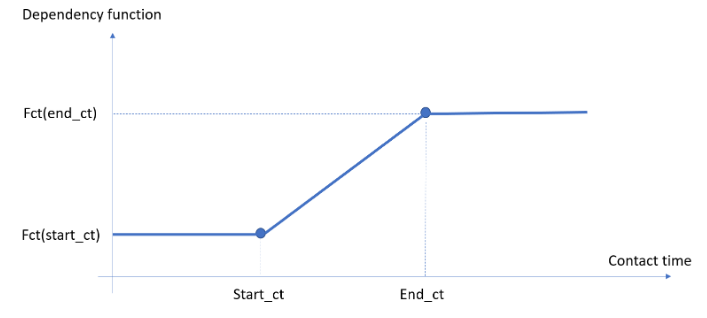
- Field
Displays the contact time.
- Start_ct
Specify the x-component of the first point of the (smoothed) ramp dependency function.
- Fct(start_ct)
Specify the y-component of the first point of the (smoothed) ramp dependency function.
- End_ct
Specify the x-component of the second point of the (smoothed) ramp dependency function.
- Fct(end_ct)
Specify the y-component of the second point of the (smoothed) ramp dependency function.
Interface boundary zone property settings for your simulation.
- Conformal Interface
Enable this option if the interface is conformal, that is, the two cell zones share the same mesh nodes along the interface.
- Type
Specify the type of interface such as Fluid-Solid, Fluid-Fluid, Solid-Solid, Fluid-Porous and Solid-Porous.
- Interface Zone
Select the zone(s) that represents the conformal interface.
- Cell Zone 1
Specify the cell zone on the first side of the (non-conformal) interface.
- Boundary Zone 1
Specify the boundary of cell zone 1 that participates in the (non-conformal) interface.
- Cell Zone 2
Specify the cell zone on the second side of the (non-conformal) interface.
- Boundary Zone 2
Specify the boundary of cell zone 2 that participates in the (non-conformal) interface
- Interface Geometries Match
If interface geometries match, all nodes of both boundaries must be part of the interface. Do not select if boundaries do not fully overlap.
- Momentum Transfer
Choose the way momentum is transferred through the interface, such as Program controlled, Bidirectional, Unidirectional, Complementary, or Filtered. Bidirectional means that constraints are written from the primary side to the secondary side and inversely. Unidirectional means that constraints are written from the primary side to the secondary side only. Complementary means that constraints are created from the secondary side to the primary side only if necessary to complement the ones written from the primary to the secondary side. Filtered means that a heuristic is used to limit the number of constraints to the necessary.
- Thermal Transfer
Choose the way thermal information is transferred through the interface, such as Program controlled, Bidirectional, Unidirectional, Complementary, or Filtered. Bidirectional means that constraints are written from the primary side to the secondary side and inversely. Unidirectional means that constraints are written from the primary side to the secondary side only. Complementary means that constraints are created from the secondary side to the primary side only if necessary to complement the ones written from the primary to the secondary side. Filtered means that a heuristic is used to limit the number of constraints to the necessary.
- Species Transfer
Choose the way species information is transferred through the interface, such as Program controlled, Bidirectional, Unidirectional, Complementary, or Filtered. Bidirectional means that constraints are written from the primary side to the secondary side and inversely. Unidirectional means that constraints are written from the primary side to the secondary side only. Complementary means that constraints are created from the secondary side to the primary side only if necessary to complement the ones written from the primary to the secondary side. Filtered means that a heuristic is used to limit the number of constraints to the necessary.
- Spreading Factor
Do not change this parameter unless requested by customer support.
- Thermal Smoothing Factor
Do not change this parameter unless requested by customer support.
- Species Smoothing Factor
Sets the numerical diffusivity included within the connected boundaries to avoid non-physical behavior. Do not change this parameter unless requested by customer support.
- Primary Side
Select the primary side of the interface for the creation of constraints. It ideally should be the side with the coarser mesh.
- Face Extension Factor
Specify a value for the face extension factor that defines the expansion of each face of the source boundary to detect the corresponding face on the target boundary. The default value is set according to the dimensions of the mesh, and it is generally not needed to modify it.
- Normal Tolerance Factor
Specify a value for the geometrical tolerance dictating the search for correspondent nodes across the interface.
- Typical Shear Rate
Specify a value for a typical shear-rate in the modelled flow. It will be used to tune the momentum transfer.
- Typical Temperature
Specify a value for a typical temperature in the model. It will be used to tune the thermal transfer.
Fluid-fluid interface boundary zone property settings for your simulation.
- Conformal Interface
Enable this option if the interface is conformal, that is, the two cell zones share the same mesh nodes along the interface.
- Type
Specify the type of interface such as Fluid-Solid, Fluid-Fluid, Solid-Solid, Fluid-Porous and Solid-Porous.
- Interface Zone
Select the zone(s) that represents the conformal interface.
- Cell Zone 1
Specify the cell zone on the first side of the (non-conformal) interface.
- Boundary Zone 1
Specify the boundary of cell zone 1 that participates in the (non-conformal) interface.
- Cell Zone 2
Specify the cell zone on the second side of the (non-conformal) interface.
- Boundary Zone 2
Specify the boundary of cell zone 2 that participates in the (non-conformal) interface
- Intersection Control
- Interface Geometries Match
If interface geometries match, all nodes of both boundaries must be part of the interface. Do not select if boundaries do not fully overlap.
- Momentum Transfer
Choose the way momentum is transferred through the interface, such as Program controlled, Bidirectional, Unidirectional, Complementary, or Filtered. Bidirectional means that constraints are written from the primary side to the secondary side and inversely. Unidirectional means that constraints are written from the primary side to the secondary side only. Complementary means that constraints are created from the secondary side to the primary side only if necessary to complement the ones written from the primary to the secondary side. Filtered means that a heuristic is used to limit the number of constraints to the necessary.
- Thermal Transfer
Choose the way thermal information is transferred through the interface, such as Program controlled, Bidirectional, Unidirectional, Complementary, or Filtered. Bidirectional means that constraints are written from the primary side to the secondary side and inversely. Unidirectional means that constraints are written from the primary side to the secondary side only. Complementary means that constraints are created from the secondary side to the primary side only if necessary to complement the ones written from the primary to the secondary side. Filtered means that a heuristic is used to limit the number of constraints to the necessary.
- Species Transfer
Choose the way species information is transferred through the interface, such as Program controlled, Bidirectional, Unidirectional, Complementary, or Filtered. Bidirectional means that constraints are written from the primary side to the secondary side and inversely. Unidirectional means that constraints are written from the primary side to the secondary side only. Complementary means that constraints are created from the secondary side to the primary side only if necessary to complement the ones written from the primary to the secondary side. Filtered means that a heuristic is used to limit the number of constraints to the necessary.
- Spreading Factor
Do not change this parameter unless requested by customer support.
- Thermal Smoothing Factor
Do not change this parameter unless requested by customer support.
- Species Smoothing Factor
Sets the numerical diffusivity included within the connected boundaries to avoid non-physical behavior. Do not change this parameter unless requested by customer support.
- Primary Side
Select the primary side of the interface for the creation of constraints. It ideally should be the side with the coarser mesh.
- Face Extension Factor
Specify a value for the face extension factor that defines the expansion of each face of the source boundary to detect the corresponding face on the target boundary. The default value is set according to the dimensions of the mesh, and it is generally not needed to modify it.
- Normal Tolerance Factor
Specify a value for the geometrical tolerance dictating the search for correspondent nodes across the interface.
- Typical Shear Rate
Specify a value for a typical shear-rate in the modelled flow. It will be used to tune the momentum transfer.
- Typical Temperature
Specify a value for a typical temperature in the model. It will be used to tune the thermal transfer.
- Fixed Part
For conformal fluid-fluid interfaces, specify the fixed part from the list of adjacent boundaries.
- Moving Interface
For conformal fluid-fluid interfaces, indicate whether the interface is in motion or not.
- Allow Non-Zero Normal Velocity
Deselecting this option forces the normal velocity to be null along the interface.
- Allow Non-Zero Tangential Velocity
Deselecting this option forces the tangential velocity to be null along the interface.
Fluid-solid interface boundary zone property settings for your simulation.
- Conformal Interface
Enable this option if the interface is conformal, that is, the two cell zones share the same mesh nodes along the interface.
- Type
Specify the type of interface such as Fluid-Solid, Fluid-Fluid, Solid-Solid, Fluid-Porous and Solid-Porous.
- Interface Zone
Select the zone(s) that represents the conformal interface.
- Cell Zone 1
Specify the cell zone on the first side of the (non-conformal) interface.
- Boundary Zone 1
Specify the boundary of cell zone 1 that participates in the (non-conformal) interface.
- Cell Zone 2
Specify the cell zone on the second side of the (non-conformal) interface.
- Boundary Zone 2
Specify the boundary of cell zone 2 that participates in the (non-conformal) interface
- Wall Condition
- Slip specification
Select the flow conditions at the wall boundary. You can choose whether to impose a zero velocity (no slip), a friction force (partial slip), or no friction (free slip)
- Slip model
For slip conditions, specify how the shear force is calculated with respect to the tangential relative velocity.
- Friction coefficient
Specify the friction coefficient for the Navier law slip conditions.
- Friction coefficient
Specify the friction coefficient for the Generalized Navier law slip conditions.
- Scaling factor
Specify the scaling factor for the Generalized Navier law slip conditions.
- Exponent
Specify the exponent for the Generalized Navier law slip conditions.
- First Friction Coefficient
Specify the first friction coefficient for the slip conditions.
- Second Friction Coefficient
Specify the second friction coefficient for the slip conditions.
- Critical stress
The critical force density at which the friction coefficient changes. When this stress is exceeded, the second friction component is used.
- First Friction Coefficient
Specify the first friction coefficient for the generalized threshold law slip conditions.
- First Scaling factor
Specify the first scaling factor for the generalized threshold law slip conditions. This scaling factor has the dimensions of the velocity, and it affects the slope of the first part the slip-velocity curve.
- Second Friction Coefficient
Specify the second friction coefficient for the generalized threshold law slip conditions.
- Second Scaling factor
Specify the second scaling factor for the generalized threshold law slip conditions. This scaling factor has the dimensions of the velocity, and it affects the slope of the second part the slip-velocity curve.
- Exponent
Specify the exponent for the generalized threshold law slip conditions.
- Friction Coefficient
Specify the friction coefficient for the asymptotic slip conditions.
- Scaling Factor
A scaling factor with the dimensions of the velocity. It affects the slope of the slip-velocity curve.
- Temperature Dependence
Specify whether the thermal dependency is a constant, or it obeys a first-order approximation of the Arrhenius law, or it obeys the Arrhenius law.
- Ea / R
Specify the ratio of the activation energy to the thermodynamic constant.
- Reference Temperature
A reference temperature for which the thermal dependency function H(T) is 1.
- Pressure Dependence
Specify the pressure dependency of the slip model along the interface as either exponential or linear.
- Alpha
Specify a value for the linear pressure dependency.
- Beta
Specify a value for the exponential pressure dependency.
Guiding device boundary zone property settings for your simulation.
- Type
Specify the guiding device type as a Conveyor belt, Single roller or Roller Conveyor.
- Enable Contact
This option is enabled by default and enables contact between the free surface and the guiding device. When disabled, the guiding device will be deactivated without deleting the guiding device boundary zone. Disabling this option can be useful as a starting point when setting up a more complex case.
- Point of Plane
Specifies the location of the conveyor belt plane.
- Px
Specify the x-coordinate of the conveyor belt plane.
- Py
Specify the y-coordinate of the conveyor belt plane.
- Pz
Specify the z-coordinate of the conveyor belt plane.
- Normal to Plane
Specify the normal to plane coordinates.
- Nx
Specify the x-component of the normal direction to the conveyor belt plane.
- Ny
Specify the y-component of the normal direction to the conveyor belt plane.
- Nz
Specify the z-component of the normal direction to the conveyor belt plane.
- Translational Velocity
Specify the velocity vector for the conveyor belt.
- Vx
Specify a value for the x-component of the translational velocity of the conveyor belt.
- Vy
Specify a value for the y-component of the translational velocity of the conveyor belt.
- Vz
Specify a value for the z-component of the translational velocity of the conveyor belt.
- Number of Rollers
Specify the number of rollers in the roller conveyor.
- Rotation-Axis Origin
Specify the coordinates of the rotation axis for the first/single roller.
- Xo
Specify the x-coordinate of the rotation-axis origin point.
- Yo
Specify the y-coordinate of the rotation-axis origin point.
- Zo
Specify the z-coordinate of the rotation-axis origin point.
- Rotation-Axis Extremity
Specify the coordinates that define the extremities of the first/single roller rotation axis.
- Xe
Specify the x-coordinate for the rotation axis extremity.
- Ye
Specify the y-coordinate for the rotation axis extremity.
- Ze
Specify the z-coordinate for the rotation axis extremity.
- Omega
Specify the angular velocity of the roller(s).
- Vector between Two Successive Rollers
Specify the components of the translation vector between two successive rollers of the roller conveyor.
- Dx
Specify the x-component of the translation vector representing the offset between two successive rollers of the roller conveyor.
- Dy
Specify the y-component of the translation vector representing the offset between two successive rollers of the roller conveyor.
- Dz
Specify the z-component of the translation vector representing the offset between two successive rollers of the roller conveyor.
- Radius
Specify the radius of the single roller or the rollers of the roller conveyor.
- Rotation-Axis Origin
Specify the coordinates of the rotation axis for the conveyor roller.
- Xo
Specify the x-coordinate of the rotation-axis origin point.
- Yo
Specify the y-coordinate of the rotation-axis origin point.
- Zo
Specify the z-coordinate of the rotation-axis origin point.
- Rotation-Axis Extremity
Specify the coordinates that define the extremities of the conveyor roller rotation axis.
- Xe
Specify the x-coordinate for the rotation axis extremity.
- Ye
Specify the y-coordinate for the rotation axis extremity.
- Ze
Specify the z-coordinate for the rotation axis extremity.
- Omega
Specify the angular velocity of the rollers.
- Contact Condition
Specify the contact conditions.
- Free Surfaces
Specify the free surfaces that will be in contact with the guiding device.
- Penetration Accuracy
Specify the penetration accuracy. If the penetration of a point into the guiding device is greater than the penetration accuracy, the time step will be rejected. The calculation will then be restarted from the previous time step with a smaller time-step increment. The default value is set according to the dimensions of the mesh, and you will generally not need to modify it.
- Slipping Coefficient
Specify a value or an expression for the slipping coefficient. If the slip coefficient and penalty coefficient have the same value and if that value is very large, then it is assumed that the fluid sticks to the guiding device when it comes into contact. Full slippage at the contact boundary is assumed if the slip coefficient is zero.
- Penalty Coefficient
Specify a value or an expression for the penalty coefficient, which enforces the condition that the fluid velocity must be equal to the guiding device velocity in the normal direction.
Point-specific pressure property settings for your simulation.
- Search Zone
Select the cell zone(s) in which the point closest to the coordinates provided below must be located.
- Pressure
Specify a value for the pressure that must be imposed at the desired point.
- X
Specify a value for the x-coordinate of the desired point for the assigned pressure.
- Y
Specify a value for the y-coordinate of the desired point for the assigned pressure.
- Z
Specify a value for the z-coordinate of the desired point for the assigned pressure.
Point-specific displacement property settings for your simulation.
Specify the components to be fixed at a specified point and their fixed displacement values.
- Search Zone
Select the cell zone(s) in which the point closest to the coordinates provided below must be located.
- Fix Dx
Enable this option to set a fixed displacement value for the x-coordinate of the solid at the desired point.
- Dx
Specify a value for the x-coordinate of the fixed displacement at the desired point.
- Fix Dy
Enable this option to set a fixed displacement value for the y-coordinate of the solid at the desired point.
- Dy
Specify a value for the y-coordinate of the fixed displacement at the desired point.
- Fix Dz
Enable this option to set a fixed displacement value for the z-coordinate of the solid at the desired point.
- Dz
Specify a value for the z-coordinate of the fixed displacement at the desired point.
Specify the point where the fixed displacement will be applied
In polymer extrusion simulations, you can specify the type of deformation to be applied to the extrudate. To cope with the displacement of free surfaces, a local mesh deformation method must be applied to the volume representing the extrudate. The purpose of a remeshing technique is to relocate internal nodes according to the displacement of boundary nodes. Remeshing techniques control mesh deformations in order to avoid unacceptable element shapes.
For polymer extrusion simulations that include a determination of the die lip shape, you can describe how the die will be deformed in the simulation using a die deformation condition. The die deformation condition is applied to a specific volume or body in the simulation that corresponds to the die. The die deformation condition applies localized remeshing to the die volume in addition to the extrudate, because the die shape is unknown beforehand and will be computed based on the given extrudate shape. Remeshing must be applied to the extrudate as well, because only the exit shape is known.
Mesh deformation methods include:
Optimesh: The Optimesh algorithm is based on a "minimum energy" rule and belongs to the family of elliptic remeshing rules and, as such, handles internal nodal displacements as variables. Optimesh is often more robust because the angular deformation of each individual element is under control of the remeshing rule.
For 3D extrusion problems, the domain is sliced in the direction of extrusion, generating a series of 2D meshes on which the Optimesh rule can be applied.
Program Controlled: Allow Fluent to choose the most appropriate remeshing technique based on the specific nature of the simulation settings.
Streamwise: The Streamwise algorithm assumes a regularity of the domain, which can be seen as a series of mesh lines emitted from the die lip section.
Along these mesh lines, which can be on the boundary, on the interface between coextruded fluids, or inside the domain, the streamwise method aligns the mesh with the local velocity vector. The method is useful in situations where large isotropic deformations occur. A typical example is 3D fiber spinning with large drawdown ratios.
Elastic: This remeshing technique belongs to the family of elliptic remeshing schemes and has the advantage of complete topological generality, since no regular organization of the mesh is required.
In the interior of the domain, a nonlinear small displacement pseudo-elastic problem is solved in the deformed configuration and not on the original domain.
This technique should not be used when the extrudate is not maintained in the extrusion direction by planes of symmetry, slipping surfaces, or rigid insert(s).
Elastic with torsion control: This is a version of the Elastic method, but with a torsion factor that adds a rotation stiffness with respect to the initial configuration. This avoids deforming elements too much with respect to their initial shape.
Property settings for the deformation zones in your simulation.
- Zones
Select the zones that belong to the same fluid cell zone where the deformation method should be applied.
- Type
Allows you to choose from a list of available deformation zones types.
- Extrudate Deformation Method
Select the deformation method to use for the extrudate such as Planes, Optimesh-3D, Streamwise, Elastic or Elastic with torsion control.
- Die Deformation Method
Select the deformation method to use for the die such as Program controlled, Sliceable (semi-structured) or Not sliceable (unstructured).
- Inlet Section
Choose a boundary for the inlet section of the extrudate remeshing zone.
- Outlet Section
Choose a boundary for the outlet section of the extrudate remeshing zone.
- Inlet Section (Constant or Adaptive Die)
For constant or adaptive die sections, specify a boundary for the inlet section of the extrudate.
- Outlet Section (Constant or Adaptive Die)
For constant or adaptive die sections, specify a boundary for the outlet section of the extrudate.
- Free Displacement on Section
Allows you to choose a list of boundary zones where mesh deformation will be free (no constraints of any type)
- No Displacement on Section
Allows you to choose a list of boundary zones where no mesh deformation will take place.
The following are properties related to adaptive remeshing.
- Enabled
Indicate whether or not to use adaptive meshing. By default, adaptive meshing is enabled (the check box is checked). You may disable it by clearing the box; this can be useful for a preliminary trial simulation. When enabled, additional properties are available.
- Number of Steps
Indicate the number of time steps to use for adaptive meshing. A value of 1 indicates that adaptive meshing will take place at each time step. Adaptive meshing is invoked after every sequence of N successful steps, by default N = 5. This is a recommended value as a good compromise between the need of best mesh quality (frequent adaptive meshing) and the necessity of speeding up the calculation (less frequent adaptive meshing). For transient cases, the value should preferably never be less than 4.
- Maximum Number of Subdivisions
Specify the number of times a primitive element. That is, an element of the initial mesh, as created in the mesh generator) can be subdivided recursively.
- Adaptive Meshing at Start
Indicate whether or not to use adaptive meshing at the start of the calculations. That is, for blow molding and thermoforming simulations that involve both contact and adaptive meshing, you can specify that an additional adaptive meshing step is performed before the start of the transient simulation. Adaptive meshing is not enabled at the start of the calculation, by default the check box is cleared. It is assumed that the initial finite element mesh is of acceptable quality, so that an initial adaption step is often not needed. If the initial mesh is of insufficient quality, you may ask for an initial mesh adaption.
- Conformalization
Indicate whether or not to use conformalization on the mesh. For 2D and shell meshes that use the recursive subdivision technique, you can enable conformalization for the mesh. For shells only, conformalization of elements is invoked by default. Adjacent elements are not always subdivided up to the same level, and two smaller elements may be adjacent to a less-subdivided element. A non-conformal situation is created where a middle mesh node may miss a contribution from the adjacent large element. This is internally solved with appropriate constraints. Alternatively, you can invoke mesh conformalization.
- Triangulation
Indicate whether to use partial or full triangulation for the mesh. If Full triangulation is used, when one element is selected for remeshing, the whole moving domain. That is, the domain for which there are local criteria activated) will be remeshed. With big meshes, the cost of this operation could be too high. Partial triangulation is when one element is selected for remeshing, a zone defined upon the neighbors of this element will be remeshed (and not the entire mesh), and is preferable for large meshes. By default, full triangulation is invoked, and is recommended unless otherwise specified. Full or partial triangulation can be invoked, respectively depending whether the adaptive meshing is applied on the entire fluid mesh or only on portions surrounding elements of bad quality.
- Angle Conservation
Enables angle conservation on the border of the remeshed zone(s). A sequence of adaptive meshing tends to erode sharp borders or edges of a fluid domain. It is especially visible on convex borders. By default, angles are not preserved. Enable this option if you want angles above a given value to be preserved and enter the value. The angle between two adjacent boundary elements is defined as the angle between vectors normal to these elements.
- Angle [deg]
Specify a value for the minimum angle that should be conserved.
- Mapping
- Enabled
Indicate whether or not to use mapping for the adaptive meshing. A mapping technique is used that projects the nodes along the local normal to the free surface, since the remeshing algorithm used for triangular / tetrahedral element generation builds a new mesh on the basis of the old mesh, rather than the original geometry.
- Planes of Symmetry Taken into Account
Indicate whether or not to account for symmetry planes. A specific mapping treatment is applied in order to preserve planes of symmetry and not geometrically distort them. By default, the option is not enabled and it is recommended unless otherwise specified.
- Threshold Value
This field triggers the mapping of the nodes. The contact algorithm uses internal fields that are named contact_field and are defined on the free surface. This field stores the contact information for each node and initially has a value of either 0 or 1. If a node of the free surface is in contact, the field value is 1, otherwise the value is 0. However, after a remeshing step, the contact_field values must be interpolated onto the newly generated mesh. After this interpolation, the contact_field values are no longer limited to being either 0 or 1, but can be intermediate values. (For example, 0.3). If a node of the free surface has a contact_field value greater than the threshold, the node is assumed to be in contact and will be mapped. The default value of the threshold is 0.8.
- Scaling Factor
This parameter is used to determine if a point on the free surface is in the vicinity of the mold surface. The distance between the free surface point and the mold surface must be less than typical_size*scaling_factor, where typical_size is the maximum size of a face (or a segment in 2D) of the mold surface. By default, the threshold is set to 0.6.
- Maximum Displacement Mode
Allows you to set the method for determining the maximum displacement of surface nodes during the mapping stage of the adaptive meshing as either Program controlled or User Value. It is the upper bound of the displacement applied to nodes that are mapped onto the contact surface. By default, the value is Program Controlled. You can change this and specify a User Value when prompted.
- User Displacement
In order to avoid highly distorted elements in the layer of elements adjacent to the free surface, the displacement of the mapped nodes is limited to this value. A good practice is to define the maximum displacement as 10 to 25 percent of the minimum element size imposed in the adaptive meshing setup. The default value is calculated from the typical mesh size.
- Penetration Tolerance
This parameter is used to provide a tolerance level for the distance between the free surface and the mold surface. If a point on the free surface is located inside the mold at a distance from the mold surface below this tolerance, the point will not be moved; otherwise the position of the point is corrected. Three options are available: a value of max displacement sets the penetration tolerance to be equivalent to the maximum displacement; a value of penetration accuracy sets the penetration tolerance to be equivalent to the minimum of the penetration accuracies; a value of user input allows you to provide your own value for the tolerance.
- User Value
Specify a value for the penetration tolerance, where it is recommended to keep the penetration tolerance to be less than or equal to the penetration accuracy.
- Criterion
- Quality
- Warning
Provides a message for defining a condition when activating an adaptive meshing criterion.
- Warning
Provides a message for activating an adaptive meshing criterion.
- Enabled
Indicate whether or not to consider the condition on the mesh quality in order to trigger adaptive meshing. You may disable it by clearing the box; this can be useful for a preliminary trial simulation.
- Quality
Specify a value for the expected quality of the mesh. A quality criterion decreasing from 1 (very good) down to 0 (very bad) is evaluated, and which incorporates geometric features such as aspect ratio, internal angles, skewness and bending. Fluid elements which do not match the required quality will be adapted. By default, a quality of 0.8 is required.
- Size
Specify a value for the expected element size of the mesh. Fluid elements which do not match the assigned size will be adapted. A default value is evaluated as a fraction of the overall geometric dimension of the mesh. It can be changed.
- Contact
- Enabled
Indicate whether or not to consider the condition on contact in order to trigger adaptive meshing. Once a contact condition is enabled (the check box is checked) additional properties are available and you may disable it by clearing the box; note that at least one condition must be enabled.
- Mold Surfaces of Contact
Select the contact zone(s) of the mold to consider for the present contact condition.
- Method
Specify the method for the local criterion: distance, curvature, or angle and curvature.
- Minimum Size
Specify the minimum size for newly created elements close to the mold boundary surface. This is the minimum side length of newly created elements, necessary for preventing the creation of a mesh that is too dense. By default, this parameter is assigned a value that is of the order of a tenth of the average edge length in the input mesh.
- Minimum Distance
Specify the minimum distance below which the minimum size is applied. This is the distance between fluid zone and mold below which new fluid elements will be created with the specified minimum size. By default, the minimum distance is set to 0.
- Maximum Size
Specify the maximum size for newly created elements far from the mold boundary surface. This is the maximum side length of newly created elements, necessary for preventing the creation of a mesh that is too coarse. By default, this parameter is assigned a value that is of the order of the average edge length in the input mesh.
- Maximum Distance
Specify the maximum distance beyond which the maximum size is applied. This is the distance between fluid zone and mold beyond which new fluid elements will be created with the specified maximum size. By default, this parameter is assigned a value that is of the order of the average edge length in the input mesh.
- Fraction of Radius of Curvature
For the curvature method, this value is dimensionless, and its default value is 0.2. Sufficiently close to the contact mold, element size will be a given fraction of the local radius of curvature, unless it hits the minimum size as lower bound. The selected default value of 0.2 suggests that about 5 fluid elements can be created for matching 1 radian (57 degrees) of a curved mold portion.
- Typical Distance to Mold
For the curvature method, this value has the units of length, and is the typical size of segments of the mesh. This is the distance between a fluid element and the mold below which mesh refinement begins. It is important to anticipate the contact, for having smaller elements before contact occurrence. By default, the value is a fraction of a typical geometric length of the input mesh.
- Coefficient of Proportionality
For the curvature method, this value has units of length. This coefficient may be interpreted as the intended size of the fluid elements when the contact occurs along a flat portion of the mold. For avoiding undesired interferences, either the Fraction of Radius of Curvature or the Coefficient of Proportionality should vanish.
- Tolerance
For the angle and curvature method, this value defines the tolerance for the contact. This is the maximum distance you would ideally like between any node of the mold and the nearest fluid element. This tolerance is used to locally calculate an ideal fluid element size, in that it could approach the mold within the stated tolerance.
- Critical Distance
For the angle and curvature method, this value has units of length, and is typically 10 percent of the typical size of the segments in the mesh. Note that a larger value results in larger areas of the fluid where the elements are subdivided, which produces higher element counts. On the other hand, if you choose a value that is too small, there may not be sufficient meshing iterations to reduce the elements to an appropriate size. To ensure that is not too small, you must account for the meshing frequency and the velocity of the parison / preform / sheet. The default for this parameter is one percent of the medium diagonal of the axis-aligned minimum box bounding the whole geometry. The critical distance corresponds to an anticipation distance from which mold angles and curvature will have a growing effect on the fluid mesh discretization. It is important to anticipate the contact, for having smaller elements before contact occurrence.
- Overlap
- Enabled
Indicate whether or not to apply the current condition on overlapping parts for adaptive meshing. When multiple conditions are defined, they may by enabled or disabled at will. Once enabled, additional options are available.
- Overlapping Parts
Select the overlapping part(s) that will be used for mesh adaption in the fluid zone.
- Unrefinement Threshold
Specify the required threshold for local mesh unrefinement. A so-called inside function (or overlapping function) is used to determine whether a fluid element is overlapped by a restrictor or a moving part, or not. It then received the value 1 or 0, respectively. For fluid elements far from the transition stripe, the function exhibits nearly no variation, and they can be selected for unrefinement if the variation is below the threshold value. By default, the threshold value is set to 0.01. The operating mode depends on the cell selection method. For the cell selection method based on inside field variation: when an element of the fluid zone is far enough from the border of the overlapping part. That is, when the corresponding overlapping or inside field exhibits small or no variation), the element can be selected for unrefinement. For the cell selection method based on average inside field values: when an element of the fluid zone is far enough from the overlapping part. That is, when the corresponding overlapping or inside field exhibits small values), the element can be selected for unrefinement.
- Refinement Threshold
Specify the required threshold for local mesh refinement. A so-called inside function (or overlapping function) is used to determine whether a fluid element is overlapped by a restrictor or a moving part, or not. It then received the value 1 or 0, respectively. For fluid elements located near or in the transition stripe, the function exhibits variation, and they can be selected for refinement if the variation is above the threshold value. By default, the threshold value is set to 0.05. The operating mode depends on the cell selection method. For the cell selection method based on inside field variation: when an element of the fluid zone is close enough to the border of the overlapping part. That is, when the corresponding overlapping or inside field exhibits large variation), the element can be selected for refinement. For the cell selection method based on average inside field values: when an element of the fluid zone is close enough to the overlapping part or overlapped. That is, when the corresponding overlapping or inside field exhibits large values), the element can be selected for refinement.
- Cell Selection Method
Specify whether the cell selection method for refinement/unrefinement is based on the variations or on the values of the overlapping or inside field. By default, the selection method for refinement and unrefinement checks the Variation of inside field versus both thresholds. Another method consists of checking the Average of inside field versus both thresholds. The behavior differs since elements overlapped by the solid part will also be refined.
- Refinement Zone
- Type
Specify the method in which you want to define the refinement zone: along boundaries, box, or sphere. For 2D cases, the box and the sphere are respectively reduced to rectangle and circle.
- Along Boundaries
- Boundary
Specify a boundary for the refinement zone. For moving zones, specify the free surface on which you want to attach the moving zone.
- Method
Specify the method of refinement along the boundary: distance, or curvature Specifying the size is similar to contacts.
- Minimum Size
Specify the minimum size for elements close to the mold boundary. This sets the minimum size for newly created elements close to the selected boundary. By default, this parameter is assigned a value that is of the order of a tenth of the average edge length in the input mesh.
- Minimum Distance
Specify the minimum distance below which the minimum size is applied. This is the distance between fluid points and selected boundaries below which new fluid elements will be created with the specified minimum size. By default, the minimum distance is set to 0.
- Maximum Size
Specify the maximum size for elements far from the mold boundary. This sets the maximum size for newly created elements beyond a given distance to the selected boundary. By default, this parameter is assigned a value that is of the order of the average edge length in the input mesh.
- Maximum Distance
Specify the maximum distance beyond which the maximum size is applied. This is the distance between fluid point and selected boundary beyond which new fluid elements will be created with the specified maximum size. By default, this parameter is assigned a value that is of the order of the average edge length in the input mesh.
- Fraction of Radius of Curvature
For the curvature method, this value is dimensionless, and its default value is 0.2. Sufficiently close to the selected boundary, element size will be a given fraction of the local radius of curvature, unless it hits the minimum size as lower bound. The selected default value of 0.2 suggests that about 5 fluid elements can be created for matching 1 rad (57°) of a curved boundary portion.
- Typical Distance to Boundary
For the curvature method, this value has the units of length. The typical depth of the zone adjacent to the boundary where elements can be remeshed based on the local curvature. By default, the value is a fraction of a typical geometric length of the input mesh.
- Coefficient of Proportionality
For the curvature method, this value has units of length. This coefficient may be interpreted as the intended size of the fluid elements along a flat portion of the selected boundary. For avoiding undesired interferences, either the Fraction of Radius of Curvature or the Coefficient of Proportionality should vanish.
- Box
- Xmin
Specify a value for the minimum position on the X axis for the refinement zone box (the X-coordinate of the lower-left-front point). The default value is 0.
- Ymin
Specify a value for the minimum position on the Y axis for the refinement zone box (the Y-coordinate of the lower-left-front point). The default value is 0.
- Zmin
Specify a value for the minimum position on the Z axis for the refinement zone box (the Z-coordinate of the lower-left-front point). The default value is 0.
- Xmax
Specify a value for the maximum position on the X axis for the refinement zone box (the X-coordinate of the upper-right-back point). The default value is 0.
- Ymax
Specify a value for the maximum position on the Y axis for the refinement zone box (the Y-coordinate of the upper-right-back point). The default value is 0.
- Zmax
Specify a value for the maximum position on the Z axis for the refinement zone box (the Z-coordinate of the upper-right-back point). The default value is 0.
- Element Size
- Size
The dimensions of the element can be either a constant or linear function of coordinates: A + B * x + C * y + D * z
- A
Specify the length of the element.
- B
A coefficient for the element size (a coefficient of the affine size function), 0 by default.
- C
A coefficient for the element size (a coefficient of the affine size function), 0 by default.
- D
A coefficient for the element size (a coefficient of the affine size function), 0 by default.
- Sphere
- Xc
Specify the X coordinate of the center of the sphere. The default value is 0.
- Yc
Specify the Y coordinate of the center of the sphere. The default value is 0.
- Zc
Specify the Z coordinate of the center of the sphere. The default value is 0.
- Diameter
Specify a value for the sphere diameter. The default value is 0.
- Element Size
- Size
The function A+Br dictates the size of the elements in that sphere versus the distance r with respect to the center.
- A
A constant coefficient for the element size in the spherical refinement zone. The default value is 0.
- B
A coefficient for the affine function for the dependence of the element size with respect to the distance from the center of the spherical refinement zone. The default value is 0.
Properties related to temperature initialization.
- Cell Zones
Specify one or more cell zones to which to assign this temperature initialization.
- Option
Specifies the temperature initialization method. Select f(X,Y,Z) to specify the coefficients of the temperature initialization equation. To initialize the temperature field using a CSV file containing a temperature profile, select Temperature profile.
- CSV File
Click the button to select the CSV file for the temperature profile.
- Field Name
Enter the name found in the CSV File for the temperature profile.
- Temperature T
Specify the coefficient of this temperature initialization equation.
- A
The first coefficient of the temperature initialization equation.
- B
The second coefficient of the temperature initialization equation.
- C
The third coefficient of the temperature initialization equation.
- D
The fourth coefficient of the temperature initialization equation.
Properties related to species initialization.
- Cell Zones
Specify one or more cell zones to which to assign this species initialization.
- Option
Specifies the species initialization method. Select f(X,Y,Z) to specify the components of the species initialization equation. To initialize the species field using a CSV file containing a species profile, select Species profile.
- CSV File
Click the button to select the CSV file for the species profile.
- Field Name
Enter the name found in the CSV File for the species profile.
- Species S
Specify the components of this species initialization equation.
- A
The first component of the species initialization equation.
- B
The second component of the species initialization equation.
- C
The third component of the species initialization equation.
- D
The fourth component of the species initialization equation.
There may be cases where you want to keep track of the value of one or more solution fields at a specific point in the domain (or at several points). You can do this by defining a probe. The probe definition will be used by the solver to save field values at specified intervals during the calculation.
Derived quantities are fields whose calculation requires the results of a previous calculation as their input. For example, the calculation of vorticity based on the known velocity field can be performed in a postprocessor.
- Shear Rate
Enable this option to create an output field to evaluate the shear rate.
- Viscosity
Enable this option to create an output field to evaluate the viscosity.
- Viscous Heating
Enable this option to create an output field containing the local intensity of viscous dissipation (heat generation by friction of fluid layers and slipping)
- Stress
Enable this option to create an output field containing the stress tensor (stresses in the fluid due to fluid deformation)
- Volume of Liquid
Enable this option to create an output field to evaluate the volume of the flow domain.
- Vorticity
Enable this option to create an output field to evaluate the vorticity.
- Mixing Index
Enable this option to create an output field to evaluate the mixing index lambda (λ)
- Rate of Deformation Tensor
Activates the calculation of the rate-of-deformation tensor D in the flow domain.
- Force
Enable this option to create an output field to evaluate the force.
- Flow Rate
Enable this option to create an output field to evaluate the flow rate.
- Heat Flux
Enable this option to create an output field to evaluate the heat flux.
- Convected Heat
Activates the evaluation of the convected heat field. Convected heat is evaluated automatically for each fluid boundary condition.
- Enable
Activates the evaluation of the uniformity of the velocity field at specified boundary(ies)
- Useful Borders
Select the boundary(ies) where the flow balance will be evaluated.
Evaluation of the extension components is available for 3D blow molding and thermoforming simulations. Two kinds of extensions can be evaluated:
Area Stretch Ratio: for each face of the fluid domain, this is the ratio of the face surface over the initial face surface (enabled by default).
Track Vectors: the local deformations of specified vectors (disabled by default).
You must specify the Initial Orientations of the vectors: initially parallel to the direction D, initially perpendicular to the direction D, initially radial from point P, initially circumferential around point P (where more than one can be selected at once). You must then specify the coordinates of the reference point P and orientation of the vector D. This is available if the domain is a shell.
- Enable
Indicate whether or not to activate the calculation of several technological measures of fluid zone deformation.
- Area Stretch Ratio
Indicate whether or not to evaluate the distribution of area stretch ratio undergone by the fluid zone, that is, the ratio of local area after deformation to initial area.
- Track Vectors
Activates the evaluation of the deformations of specified vectors in the flow domain.
The reference point for the extension derived quantity. You must specify the coordinates of the reference point P.
- Px
Specify the x-coordinate of the reference point P.
- Py
Specify the y-coordinate of the reference point P.
- Pz
Specify the z-coordinate of the reference point P.
The reference vector direction for the extension derived quantity. You must specify the orientation of the vector D.
- Dir-x
Specify the x-component of the reference direction D.
- Dir-y
Specify the y-component of the reference direction D.
- Dir-z
Specify the z-component of the reference direction D.
For blow molding and thermoforming processes in shell models, there are times when self-contacts such as folds or knit-lines can occur in the blown part. In such cases, the self-contact postprocessor can simply detect self-contact of the parison.
- Enable
Activates the detection of folds or knit-lines that can occur in a blown/thermoformed part.
- Action
Select the action to be taken when self-contact is detected such as No action, Warning or Stop. No action simply allows to postprocess the self-contact field. Warning generates a message in the transcript. Stop halts the calculation.
This postprocessor is available for boundaries of fluid zones in thermal simulations. Only boundaries with non-zero normal velocity should be considered. Indeed, along walls or plane of symmetries, the convected heat should be zero.
The convected heat postprocessor computes the integral along selected boundaries of  , where
  is the temperature.
- Convected Heat
Activates the evaluation of the convected heat field. Convected heat is evaluated automatically for each fluid boundary condition.
Residence time of fluid points entering the fluid domain (disabled by default). This is available if the domain is not shell and if there is at least one inlet fluid boundary condition. You must specify the fluid boundaries where it will be initialized and provide the initial value.
- Enable
Activates the evaluation of the residence time in the flow domain.
- Inlet Boundary
Select the boundary(ies) where the residence time is imposed.
- Law
Select the law for imposing the residence time such as Constant or Polynomial.
- A
Specify a value for the constant coefficient of the residence time function at the inlet boundary.
- B
Specify a value for the X coefficient of the polynomial function for the residence time function at the inlet boundary.
- C
Specify a value for the Y coefficient of the polynomial function for the residence time function at the inlet boundary.
- D
Specify a value for the Z coefficient of the polynomial function for the residence time function at the inlet boundary.
This is available if the domain is not a shell and if there is at least one inlet fluid boundary condition. In addition, you should specify the fluid boundaries where it will be initialized it and specify the initial value.
- Enable
Activates the tracking of material particles.
- Inlet Boundary
Select the boundary(ies) where the material property is imposed.
- Law
Select the law for imposing the material property such as Constant or Polynomial.
- A
Specify a value for the constant coefficient of the material property function at the inlet boundary.
- B
Specify a value for the X coefficient of the polynomial function for the material property function at the inlet boundary.
- C
Specify a value for the Y coefficient of the polynomial function for the material property function at the inlet boundary.
- D
Specify a value for the Z coefficient of the polynomial function for the material property function at the inlet boundary.
Evaluation of the thickness of a product. This is available if the domain is not a shell and not a film, and if the simulation is transient with no restrictors or moving parts. (disabled by default)
In 2D as well as in 3D simulations of blow molding and pressing, you can compute the thickness of the final object (as well as during shaping). In industrial processing, the thickness has to be understood as the distance between two arbitrary surfaces; it is therefore subjected to an appropriate definition. Also, from the point of view of modeling, it would require the identification of preferably distinct topological entities; however this cannot always be achieved. A technique has been implemented, which matches a reasonable industrial definition as much as possible: at a given point, it basically consists of evaluating the distance with respect to the closest opposite surface. A topological object has to be constructed for the thickness evaluation, and a few parameters for geometric tolerances have to be given. In 3D, the thickness is evaluated on the selected boundary; planes of symmetry can be discarded from the domain of evaluation. Note that in 2D, a similar scenario applies; however, since the display of a quantity along a line is not easy, the evaluation is expanded onto the domain via a Laplace equation.
Typically, the thickness at the end of the process is of interest. Hence, it is not necessary to perform a thickness evaluation at each time step. Also, since the thickness at a point is evaluated as a distance measured along a line perpendicular to the surface at this point, it is preferable to bound its value.
- Zones
Select the zone(s) where the derived quantity must be calculated.
- Useful Borders
Specify the border that is used as the basis for the evaluation of the thickness; it may consist of one or several boundaries, but typically symmetry planes and lines are not considered.
- Activation Time
Specify a value for the activation time. The thickness evaluation will be performed only when the simulation time is greater than or equal to the activation time.
- Tolerance
Specify a value for the geometric tolerance. The thickness at a point is evaluated as a distance between the point and the opposite surface, measured along a line perpendicular to the surface at this point. The algorithm involves a search of geometric intersection (between the perpendicular line and boundary elements). A geometric tolerance is needed in order to compensate for round-off errors.
Numerical methods affect your simulation's convergence speed as well as accuracy and stability of the solution.
- Upwinding in energy equation
Activates the upwinding numerical method on the energy equation to aid in solution convergence.
- Upwinding on free surfaces
Activates the upwinding numerical method on free surfaces to aid in solution convergence.
- Upwinding on Species
Activates the upwinding numerical method on species to aid in solution convergence.
- Decouple computation of temperature
Decouples the calculation of temperature to produce a stabilizing effect in some cases.
- Decouple Computation of Viscoelastic Stresses
Decouples the calculation of viscoelastic stress to produce a stabilizing effect in some cases (the solver updates the viscoelastic stresses fields after calculation of the velocities)
- Decouple computation of free surfaces
Decouples the calculation of free surfaces to produce a stabilizing effect in some cases.
- Decouple Computation of Species
Decouples the calculation of species to produce a stabilizing effect in some case.
- Integration method on free surfaces
Choose the type of integration for the free surface: program controlled, line integration, or surface integration.
- Integration Rule for Transient Terms
Allows you to select standard or hybrid integration rule for transient terms. The hybrid integration rule is recommended for transient thermal flow or heat conduction problems involving thermal shocks. (For example, a glass pressing problem)
- Picard iterations
Assists in the robustness of the calculation. Recommended when the selected viscosity model exhibits important variations.
- Pressure stabilization
Smooths the pressure over elements by introducing a slight compressibility of the fluid. Mandatory when using linear interpolation of velocities.
- Relative compression factor
The amount of compressibility for the pressure stabilization. A factor that is too small will introduce pressure peaks. If the factor is too large, the fluid is too compressible and all pressure gradients will be smoothed out, leading to an unrealistically low pressure prediction.
- Fluid fractions diffusivity
Specify the diffusivity for the fluid fractions.
- Overlap threshold
Specify a value of the overlap threshold that is used to separate the nodes that are inside and outside the moving parts. In general, there is no reason to modify the default value that is 0.6.
- Allow Multiple Overlapping
Allows overlapping of moving parts, a fluid node may then be inside more than one moving part.
- Slip stabilization factor
A stabilization factor for slip conditions that helps resolve problems that arise from conflicting boundary conditions.
- Advanced Volume Conservation
Enable this to enhance volume conservation in the calculations involving adaptive meshing.
The DEVSS method consists of adding a purely viscous term into the momentum equation that is expressed in terms of velocity unknowns, and removing an equivalent contribution expressed in terms of rate-of-deformation unknowns. Such a formulation keeps the constitutive equation unchanged.
- Numerical Parameters for DEVSS
Allows you to switch between Program controlled and User specified numerical parameters.
- Numerical Viscosity for DEVSS
Specify a value for the numerical viscosity which can possibly be adjusted in order to compensate for the discarded stress components.
The interpolation of a field defines the way it is represented. One can have one value per element/cell, one value per node in case of linear interpolation, or one value per node/edge/face/cell in case of quadratic interpolation.
The different interpolations for the different fields cannot be chosen completely arbitrarily. The Fluent Materials Processing workspace proposes only sensible choices.
- Coordinates
Choose the interpolation of the coordinates field. This interpolation should be linear.
- Thickness
Choose the interpolation type used to calculate the thickness field.
- Velocity (V) and pressure (P)
Choose a combination of velocity-pressure interpolations. The default is linear velocity with constant-per-element (stabilized) pressure (usually the least computationally expensive combination) . The quadratic velocity with linear pressure is the most computationally accurate and expensive.
- Stress
Choose an interpolation type used to calculate the stress field.
- Temperature
Choose an interpolation type used to calculate the temperature field, based on the Péclet number or expected temperature gradients.
- Species
Choose an interpolation type used to calculate the species field.
- Pressure at slip wall
Choose an interpolation type used to calculate the pressure applied along a slipping wall to enforce the zero normal velocity condition.
- Displacement
Choose an interpolation type used to calculate the displacement of an elastic solid.
Numerics settings related to calculating the solution for fluid-structure interaction (FSI).
- Penalty Coefficient
Specify a value for the fluid-structure interaction penalty coefficient. This enforces the condition that the fluid velocity must be equal to the wall velocity of the elastic solid, in the normal direction. The value for the penalty coefficient should only be changed to account for fluid slip on the solid surface.
- Stability Coefficient
This value should only be changed if the fluid sticks to the solid surface. The stability coefficient can be modified to prevent problems from occurring during the calculation when the fluid sticks to the solid surface at points where the velocity is already imposed. The stability coefficient is dimensionless and the value must be small with respect to 1.
Numerics settings related to free jet stabilization.
- Stabilization
Select the method for stabilizing the free jet as Program Controlled, Whole, Partial, or No. Program controlled is the default method and is sufficient for most cases. Program controlled will automatically determine if it is necessary and possible to stabilize the free jet. Additionally, values of the numerical parameters involved are determined automatically as well. When Whole is selected, the whole free jet will be stabilized. When Partial is selected, only the portion of the free jet that is adjacent to the extrudate exit will be stabilized. For both the Whole and Partial stabilization methods, if stabilization is not possible or not necessary, stabilization will be cancelled and a message will be printed in the console during the calculation. When No is selected, the free jet will not be stabilized. This can lead to unphysical deformations of the free jet if the flow field in the die end is not well balanced. However, including gravity effects and guiding device boundary conditions may resolve instability.
- Relative Tolerance on Distance
This parameter determines if the vertex of a boundary is located or not in a plane for the Whole and Partial stabilization methods. This parameter should not be modified unless requested by customer support.
- Tolerance on Plane Coefficient
This parameter allows for the coefficients of an equation of a plane to be rounded to zero for the Whole and Partial stabilization methods. This parameter should not be modified unless requested by customer support.
- Relative Starting Coordinate
When using the partial stabilization method, specify the portion of the free jet that will not be stabilized. The range must be between 0 and 1 and is set to 0.5 by default. A value of 0.25 will not stabilize 25 percent of the free jet (the portion adjacent to the die end), while a value of 0.75 will stabilize 25 percent of the free jet (the part adjacent to the extrudate exit)
The way contact is managed in the solver, a fluid node always slightly enters into the solid/mold. Parameters are set to correctly detect and limit this penetration.
- Penetration Accuracy
If the penetration of a point into the mold is greater than the penetration accuracy, the time step will be rejected. The calculation will then be restarted from the previous time step with a smaller time-step increment. The default value is set according to the dimensions of the mesh, and you will generally not need to modify it.
- Element Dilatation
This option allows for expansion of each finite element of the mold in order to help the contact detection algorithm. Some numerical errors can cause a point to "miss" the mold. A typical case can occur when a point of the fluid domain is supposed to come into contact with a mold at the location of the symmetry line of the mold. A small expansion of the finite elements fixes the problem. The default value is set according to the dimensions of the mesh, and you will generally not need to modify it.
- Search Settings
You have the choice of five predefined groups of search settings. The groups can be “faster”. That is, result in faster computation times for the search) or "safer". That is, conduct searches that are more thorough but require more computation time). By default, a fast group of settings is selected, as this group is appropriate for a relatively broad range of cases.
- Search Sector Divisions per Axis
Allows you to modify the search sector division along each Cartesian axis. In order to speed up the search of contact, the search zone is divided into N sectors along each Cartesian axis, that is, the search zone is divided into N^3 search sectors. The actual search occurs in the sector that contains the point of interest. The larger sector divisions, the faster search in a specific sector but a greater risk of missing something.
- Expansion of Search Zone
Allows you to modify the expansion of the search zone. This expansion is a increment to the dimension of the Cartesian box that surrounds the whole mold. This increment is expressed in a percentage of the largest dimension of that box.
- Overlap of Sectors
Allows you to modify the overlap of search sectors. Using overlapping sectors decreases the risk of overlooking (large) finite elements on the border of contiguous sectors. The larger the overlap, the safer search but a more expensive search in a given sector.
- Action if Limits Exceeded
Specify what actions to take if local element distortion limits are exceeded.
- Minimum Angle [deg]
Specify a value for the minimum interior angle to avoid local distortions to the mesh.
- Maximum Angle [deg]
Specify a value for the maximum interior angle to avoid local distortions to the mesh.
- Maximum Aspect Ratio
Specify a value for the maximum aspect ratio to avoid local distortions to the mesh.
- Maximum Bend
Specify a value for the maximum bend to avoid local distortions to the mesh.
- Maximum Skew
Specify a value for the maximum skew to avoid local distortions to the mesh.
- Reduction Rate of Time Step
For transient calculations, specify a value for the time step reduction rate. This is a factor that multiplies the current time step when a significant risk of element distortion is detected.
Controls the convergence and divergence criteria and the numerical progression of the polymer simulation.
- Iterations Criterion
Allows you to switch between Program controlled and User specified parameter.
- Maximum Number of Iterations
Specify a value for the maximum number of solver iterations in a given equations system resolution.
- Convergence criterion
Controls when the convergence to a stable solution is assumed. Allows the program to check convergence of the solution, or define your own criterion.
- Convergence tolerance
Specify the tolerance for when the solution is converging. When the relative variation of the solution is smaller that the provide tolerance, convergence is assumed.
- Divergence criterion
Controls the solution when divergence is assumed. Allows the program to check divergence of the solution, or define your own criterion.
- Divergence tolerance
Specify the maximum value for the relative variation of the solution at which the solver assumes divergence and stops the iterations.
- Use double-precision buffer
Determine whether or not to use double-precision buffering in your solution.
- Solver unit system
Sets the units in which all data will be converted before being passed to the solver. Setting this avoids very large or very small numbers in the solver and enhances accuracy.
- Solver type
Sets the method for solving the system of equations. Program controlled is the default, which uses the AMF direct solver for most cases. The MUMPS direct solver can be selected for large cases, such as large 3D extrusion problems or large 3D problems with contact. The AMF direct solver + secant or the MUMPS direct solver + secant options can be selected to use the secant technique: this technique has shown to work for most problems with potentially significant savings. However, in rare cases, the secant iteration may direct iterations along a wrong path and therefore this technique is not the default.
- Restart Options
- Restart Type
Allows you to select the restart option such as No previous solution, Restart from an old result file, Restart from an old CSV file or Restart from old result and restart files (non steady calculations only). When there is no previous solution, the initial state is all fields is set to zero except for those with an explicit initialization as to the temperature. An old result file is a Polyflow format file that must be topologically compatible. A CSV file that contains a cloud of data points does not require such compatibility. A restart file contains time derivatives that permit to pursue the time integration.
- RES Filename
In order to specify the pathname of the file containing calculation results in a Polyflow format, click on the Load Result File button at the bottom of the property panel.
- CSV Filename
In order to specify the pathname of the file containing calculation results in a CSV format, click on the Load CSV File button at the bottom of the property panel.
- RST Filename
In order to specify the pathname of the file containing time derivatives of a previous calculation, click on the Load Restart File button at the bottom of the property panel.
- Launch Options
- Solver arguments
Advanced command-line options (should not be used unless recommended by ANSYS Customer Support)
- Solver keywords
Advanced options (should not be used unless recommended by ANSYS Customer Support)
- Number of processors
Indicate the number of processes to use in the calculation. By default, the solver uses 4 processors.
- GPU
Allows you to activate usage of Graphical Processor Unit(s) that speed(s) up the calculation.
- Number of GPUs
Specify the number of GPUs to be used in the calculation. More than one GPU allows you to balance the load in a parallel calculation.
- Transient Controls
- Initial time step
Specify a value for the initial time step size for the transient calculations.
- Minimum time step
Specify a value for the minimum time step size for the transient calculations.
- Maximum time step
Specify a value for the maximum time step size for the transient calculations.
- Integration scheme
Choose an integration scheme for the transient calculations: Zero order, Implicit Euler, Galerkin, or Crank-Nicolson
- Tolerance
Specify a tolerance value for the transient calculations.
- Use velocity for precision evaluation
Determine whether or not you want to use velocity prediction.
- VOF Transient Controls
- Initial Time Step
Specify a value for the initial time step size for the volume of fluid transient calculations.
- Minimum Time Step
Specify a value for the minimum time step size for the volume of fluid transient calculations.
- Maximum Time Step
Specify a value for the maximum number of time steps for the volume of fluid transient calculations.
- Maximum Number of Time Steps
Specify a value for the maximum number of time steps for the transient calculations.
- Accuracy
Controls the accuracy of the scheme. Recommended values of are on the order of 0.2-0.5. Note that an extremely low value of this parameter can reduce the time step to such a degree that the fluid front does not progress anymore. Consequently, the time step will be increased and you then run the risk of engaging in an oscillatory forward/backwards marching scheme that calculates several useless iterations without improved accuracy. An inherent limitation of the VOF model is that it cannot process changes that are smaller than the element size.
- Filtering Threshold on Fluid Fraction
Some variations of the fluid fraction in the wet zone (far from interface with dry zone) may be filtered with this parameter: all variations higher than this threshold will be smoothed. The variations smaller than the threshold will be unchanged. For example, with a threshold of 0.1, if the local value of the Fluid Fraction is 0.95 (instead of 1.0 ideally), then the variation = 0.05 (= 1.0 - 0.95) is below the threshold. Consequently, the value is unchanged. However, for a value of 0.89 (instead of 1.0 ideally), then the variation = 0.11 (= 1.0 - 0.89) is above the threshold. Consequently, the value will be filtered (value reset to 1.0)
- Stop Run When Cavity Full
By default, the VOF calculation is stopped when the geometry is completely covered by the fluid or when the net flow rate (volume of fluid entering the geometry per unit of time minus volume of fluid exiting the geometry per unit of time) is zero. Disabling this criterion lets the run to reach the final time.
- Continuation Controls
- Initial Value
Specify a value for the first step of the continuation calculations.
- Upper Limit
Specify a value for the final step of the continuation calculations.
- Initial step size
Specify a value for the initial continuation step size.
- Minimum step size
Specify a value for the minimum continuation step size.
- Maximum step size
Specify a value for the maximum continuation step size.
- Maximum number of steps
Specify a value for the maximum number of continuation steps.
- Integration scheme
Choose an integration scheme for the continuation calculations: Zero order, Implicit Euler, Galerkin, or Crank-Nicolson
- Convergence Strategies
- Multiple Materials
Enable this option to assist converging flows with more than one material.
- Free Surfaces and Moving Interfaces
Enable this option to assist converging free surface flows involving a pulling component, such as take-up velocity, take-up force or gravity.
- Viscosity and Slip
Enable this option to assist converging flows with non-linear viscosity and/or slipping.
- Viscoelasticity
Enable this option to assist converging flows with viscoelastic non-linearities that often originate from the combination of high stress values developing in the vicinity of geometric singularities and of transport mechanisms inherent to viscoelasticity.
- Thermal Effects
Enable this option to assist converging flows when temperatures are important.
- Flow at Inlet
Enable this option to assist converging flows based on the flow at the inlet. Linearly increases the mass flow rate/volume flow rate/normal velocity, starting from 0 to reach the assigned value at the end of the continuation scheme.
- Flow at Outlet
Enable this option to assist converging flows based on the flow at the outlet. Linearly increases the mass flow rate/volume flow rate/normal velocity, starting from 0 to reach the assigned value at the end of the continuation scheme.
- Take-Up at Extrudate Exit
Enable this option to assist converging flows based on a take-up velocity/force/force density applied on an extrudate exit. Linearly increases the velocity/force/force density, starting from 0 to reach the assigned value at the end of the continuation scheme.
- Foaming
Enable this option to assist converging flows based on foaming.
- Fluid Structure Interaction (FSI)
Enable this option to assist converging flows with fluid-structure interaction.
Indicate specifics for the output of the material processing simulation. For example, you can specify how verbose you would like the output transcript to be, along with specifying various derived quantities that the simulation can provide.
- Output at Initial State
Specify how you will save the initialized state of the simulation (state prior to beginning the calculation). This allows you to check the initialization state of an old results file and is useful for both transient and continuation type simulations.
- Output Frequency (continuation)
Specify how often the output will be generated for continuation calculations.
- Output Frequency (transient)
Specify how often the output will be generated for transient calculations.
- Number of Steps
Specify the number of steps after which the output will be generated.
- Time Interval
Specify the time interval for the output generation.
- Step Interval
Specify the step interval for the output generation.
- Transcript Verbosity
Specify how verbose you would like the output transcript to be.
- Fields Visualization
Specify whether to include special output fields along with standard output fields.
- STL
Creates output containing the facets describing the boundaries of the domains of the geometry, such that each boundary of each region corresponds to a STL solid.
- CFD-Post
Creates output that contains the geometry and the computed fields for use with ANSYS CFD-Post.
- Polyflow
Creates output files (res.msh, res) that contain the mesh and the computed fields for use with ANSYS Polyflow. This format can also be read into the Fluent Materials Processing workspace.
- CSV
Creates this output file (csv) is a common format for tabulated data that can be read into spreadsheet programs as Excel. It can also be read in ANSYS Polyflow for initial or boundary conditions.
- EnSight
Creates output that contains the geometry and the computed fields for use with EnSight. By default, results are always available in this format as they are required by the workspace for visualizing results.
- FieldView
Creates output that contains the geometry and the computed fields for use with FieldView.
- Ansys Mapper
Creates output that contains the geometry and the computed fields for use with Ansys Mapper.
- Velocity convergence
Monitor the convergence of the velocity residuals.
- Pressure convergence
Monitor the convergence of the pressure residuals.
- Temperature convergence
Monitor the convergence of the temperature residuals.
- Species convergence
Monitor the convergence of the species residuals.
- Stress convergence
Monitor the convergence of the stress residuals.
- Thickness convergence
Monitor the convergence of the thickness residuals.
- Coordinates Convergence
Monitor the convergence of the coordinates residuals.
- Fluid Fraction Convergence
Monitor the convergence of the fluid fraction residuals.
- Density Convergence
Monitor the convergence of the fluid density in foaming flows.
- Bubble Radius Convergence
Monitor the convergence of the bubble radius in foaming flows.
- Displacement Convergence
Monitor the convergence of the displacement residuals.
Allows you to create a new point surface.
- X
Specify the x-component of the point location.
- Y
Specify the y-component of the point location.
- Z
Specify the z-component of the point location.
Allows you to create a new line surface.
- First Point
- X
Specify the x-component of the first point of the line.
- Y
Specify the y-component of the first point of the line.
- Z
Specify the z-component of the first point of the line.
- Second Point
- X
Specify the x-component of the second point of the line.
- Y
Specify the y-component of the second point of the line.
- Z
Specify the z-component of the second point of the line.
Allows you to create a new rake surface.
- Number of Points
Specify the number of points to have as part of the rake surface.
- Start Point
- X
Specify the x-coordinate of the starting point of the rake surface.
- Y
Specify the y-coordinate of the starting point of the rake surface.
- Z
Specify the z-coordinate of the starting point of the rake surface.
- End Point
- X
Specify the x-coordinate of the ending point of the rake surface.
- Y
Specify the y-coordinate of the ending point of the rake surface.
- Z
Specify the z-coordinate of the ending point of the rake surface.
Allows you to create a new plane surface.
- Creation Mode
Choose how the plane should be created. A plane can be created using Three Points, using a Point and Normal vector, or by specifying the XY, YZ, or ZX planes.
- Bounded
Select to have your plane bounded by the extents of the domain.
- X
Specify the x-coordinate of the point in the plane creation.
- Y
Specify the y-coordinate of the point in the plane creation.
- Z
Specify the z-coordinate of the point in the plane creation.
- Point 0
- X
Specify the x-coordinate of the first point in the plane creation.
- Y
Specify the y-coordinate of the first point in the plane creation.
- Z
Specify the z-coordinate of the first point in the plane creation.
- Point 1
- X
Specify the x-coordinate of the second point in the plane creation.
- Y
Specify the y-coordinate of the second point in the plane creation.
- Z
Specify the z-coordinate of the second point in the plane creation.
- Point 2
- X
Specify the x-coordinate of the third point in the plane creation.
- Y
Specify the y-coordinate of the third point in the plane creation.
- Z
Specify the z-coordinate of the third point in the plane creation.
- Normal
- X
Specify the x-component of the vector in the plane creation.
- Y
Specify the y-component of the vector in the plane creation.
- Z
Specify the z-component of the vector in the plane creation.
Allows you to create a new iso-surface.
- Field
Select the field variable that you want to use for creating the iso-surface.
- Iso Value
Specify a value to apply to the iso-surface.
- Minimum
The minimum value of the selected field.
- Maximum
The maximum value of the selected field.
- Restrict To Specific Surfaces
Select to restrict the iso-surface to a particular surface.
- Surfaces
Select the surface(s) that you want to restrict to the iso-surface.
- Restrict To Specific Zones
Select to restrict the iso-surface to a particular zone.
- Zones
Select the zone(s) that you want to restrict to the iso-surface.
Allows you to create a new iso-clip.
- Field
Select the field variable that you want to use for creating the iso-clips.
- Surfaces
Select the surface(s) that you want to apply to the iso-clip.
- Minimum
Specify a minimum iso-clip value.
- Maximum
Specify a maximum iso-clip value.
Allows you to set properties for your report definitions.
- Name
Specify a name for the report, or use the default name.
- Type
Choose the type of report as either a surface report or a volume report.
- Quantity
Choose the surface or volume quantity that you want to report.
- Field
Select the field variable to be used in the surface or volume integrations.
- Surfaces
Select the surfaces used in computing the report definition.
- Volumes
Select the volumes used in computing the report definition.
- Per Surface
Select to include individual surfaces or volumes.
When the Type is set to Surface, you can obtain a report for selected surfaces of various quantities of a specified field variable
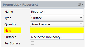
Surface reports can be created for a specific Quantity, including:
Area—area of the selected surfaces.
Area Average—area-weighted average of the specified variable over the selected surface(s).
Facet Average—facet average of the specified variable over the selected surface(s).
Facet Minimum—facet minimum of the specified variable over the selected surface(s).
Facet Maximum—facet maximum of the specified variable over the selected surface(s).
Flow Rate—flow rate of the specified variable over the selected surface(s).
Surface Integral—surface integral of the specified variable over the selected surface(s).
Surface Mass Average—mass average of the specified variable over the selected surface(s).
Mass Flow Rate—mass flow rate of the specified variable over the selected surface(s).
Standard Deviation—standard deviation of the specified variable over the selected surface(s).
Surface Sum—sum of the specified variable over the selected surface(s).
Vertex Average—vertex average of the specified variable over the selected surface(s).
Vertex Minimum—vertex minimum of the specified variable over the selected surface(s).
Vertex Maximum—vertex maximum of the specified variable over the selected surface(s).
Volume Flow Rate—volume flow rate of the specified variable over the selected surface(s).
When the Type is set to Volume, you can obtain a report for selected volumes of various quantities of a specified field variable
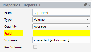
Volume reports can be created for a specific Quantity, including:
Average—averaged value of the specified variable across the domain.
Volume Integral—volume integral of the specified variable over domain.
Volume Mass Average—volume-averaged value of the specified variable across the domain.
Mass Integral—mass-weighted integral of the specified variable across the domain.
Volume—volume of the domain.
Maximum—maximum value of the specified variable over the domain.
Minimum—minimum value of the specified variable over the domain.
Volume Sum—sum of the specified variable over the domain.
Mass—mass of the entire domain.
Allows you to create new, or edit existing LIC settings objects.
- Vector Field
Choose an existing vector variable to display on the surface.
- Contrast
Select to do a pass of image contrast enhancement.
- Length
Specify a maximum length of 20 pixel units in the positive and negative directions. Length is a scaling factor of this 20 pixels. Range is 0 to 1.
- Integration Step
Specify the step size in pixel units for each integration step. Range is 0 to 1.
- Brightness
Specify the surface brightness. Range is 0 to 1.
Allows you to create new, or edit existing mesh objects.
- Shrink Factor
Specify a value for the mesh shrink factor. To distinguish individual faces or cells in the display, enlarge the space between adjacent faces or cells by increasing this value.
- Surfaces
Select the surface(s) where you want to display the mesh.
- Display LIC
Select to display the line integral convolution.
- Options
- Nodes
Select to include nodes in the mesh display.
- Edges
Select to include edges in the mesh display.
- Faces
Select to include faces in the mesh display.
- Edge Options
- Type
Choose how the edges will be displayed, all edges, edges within a specific feature angle, or just the outline.
- Feature Angle
Specify a value for the edge feature angle to control how you can display certain features in complex geometries.
- Coloring
- Automatic
Select to use automatic mesh coloring, where the coloring is automatically determined by either boundary type or ID. If disabled, you can color faces, edge, and node independently.
- Color By
Specify whether to automatically color the mesh by boundary type or by boundary ID.
- Color Faces By
Specify a color to apply to faces.
- Color Edges By
Specify a color to apply to edges.
- Color Nodes By
Specify a color to apply to nodes.
Allows you to create new, or edit existing contour objects.
- Field
Select the field variable that you want to use for creating the contour plot.
- Surfaces
Select the surface(s) where you want to display the contour plot.
- Display Filled Contour
Select to visualize the contour plot using filled contours.
- Display LIC
Select to display the line integral convolution.
- Contour Lines
Select to visualize the contour plot using just contour lines.
- Coloring
Choose whether you want a smooth, transitional display of contours or a delineated, banded display of contours.
- Draw Mesh
Enable to draw the mesh with the contours.
- Range
- Auto-Compute Range
Select to automatically determine the range of contour values.
- Global Range
Select to have the contour display use data from the entire domain.
- Clip To Range
Select to have the contour display use data from a specific portion of the domain defined by specified minimum and maximum values.
- Minimum Value
Specify a minimum value for the contour data.
- Maximum Value
Specify a maximum value for the contour data.
- Color Map
- Visible
Select to have the color key displayed along with the contour display.
- Size
Specify the number of distinct color intervals in the color scale (especially applicable for banded contour displays) or keep the default value. Values from 2 to 100 are acceptable, where increments of 10 are recommended.
- Color Map
Select a particular contour color map scheme, or keep the default selection.
- Use Log Scale
Select to have the contour display use a logarithmic scale.
- Position
Choose the position of the contour color map in the graphics window, or use the default value.
- Type
Choose the contour color map presentation of data as general, exponential, or float.
- Precision
Specify the numerical precision for the contour color map data.
- Automatically Skip Labels
Select to skip a certain number of labels (or show all) in the contour color map.
- Skip
Specify the number of color levels to include in the contour color map.
Allows you to create new, or edit existing vector objects.
- Vector Field
Select the vector quantity to be plotted.
- Field
Select the field variable that you want to use for creating the vector plot.
- Surfaces
Select the surface(s) where you want to display the vector plot.
- Skip
Specify the number of levels to include in the vector plot.
- Style
Select a particular style for your vector markers.
- Draw Mesh
Enable to draw the mesh with the vectors.
- Range
- Auto-Compute Range
Select to automatically determine the range of vector values.
- Global Range
Select to have the vector display use data from the entire domain.
- Clip To Range
Select to have the vector display use data from a specific portion of the domain defined by specified minimum and maximum values.
- Min Value
Minimum Value
- Max Value
Maximum Value
- Color Map
- Visible
Select to have the color key displayed along with the vector display.
- Size
Specify the number of distinct color intervals in the color scale or keep the default value. Values from 2 to 100 are acceptable, where increments of 10 are recommended.
- Color Map
Select a particular vector color map scheme, or keep the default selection.
- Use Log Scale
Select to have the vector display use a logarithmic scale.
- Position
Choose the position of the vector color map in the graphics window, or use the default value.
- Type
Choose the vector color map presentation of data as general, exponential, or float.
- Precision
Specify the numerical precision for the vector color map data.
- Automatically Skip Labels
Select to skip a certain number of labels (or show all) in the vector color map.
- Skip
Specify the number of color levels to include in the vector color map.
- Vector Options
- In Plane
Select to display the vector in the plane normal to the flow.
- Fixed Length
Select to have all of the vectors displayed with the same length.
- X Component
Select to include the x-component of the vector.
- Y Component
Select to include the y-component of the vector.
- Z Component
Select to include the z-component of the vector.
- Head Scale
Specify a value that can control the size of the arrowhead for the vector display.
- Color
Choose a color for the vector arrows.
- Scale
- Auto Scale
Select to use automatic scaling in the vector display.
- Scale
Specify a value in order to increase or decrease the vector scale from the default auto scale value.
Allows you to create new, or edit existing pathline objects.
- Vector Field
Select the vector quantity to be plotted.
- Steps
Specify the maximum number of steps a particle can advance. A particle will stop when it has traveled this number of steps or when it leaves the domain.
- Path Density
Specify the density of pathlines for better visualization.
- Color by
Select the field variable to be used to color the pathlines.
- Release from Surfaces
Select the surface(s) from which the pathlines will be originating.
- Draw Mesh
Enable to draw the mesh with the pathlines.
- Options
- Oil Flow
Select to display pathlines that are constrained to lie on a particular boundary.
- Reverse
Select to reverse the direction of the pathlines display.
- Node Values
Select to use values that have been interpolated to the nodes, or computed cell-center values in the pathlines plot.
- Relative
Display the pathlines relative to the rotating reference frame.
- Range
- Auto-Compute Range
Select to automatically determine the range of pathline values.
- Minimum Value
Specify a minimum value for the pathline data.
- Maximum Value
Specify a maximum value for the pathline data.
- Style
- Style
Choose from a variety of styles to apply to your pathline display.
- Line Width
Specify the width of an individual pathline.
- Arrow Space
Specify the space between the line-arrow pathlines.
- Arrow Scale
Specify the size of the line-arrow pathline.
- Marker Size
Specify the size of the marker when using marker pathlines.
- Diameter
Specify the diameter of the sphere when using sphere pathlines.
- Radius
Specify the radius of the sphere when using sphere pathlines.
- Width
Specify the thickness of pathlines.
- Accuracy Control
- Accuracy Control On
Select to mitigate any potential accuracy issues for pathline calculations when using large time step sizes.
- Minimum Steps
Specify the minimum number of steps a particle can advance.
- Maximum Steps
Specify the maximum number of steps a particle can advance.
- Maximum Angle
Specify the maximum angle of a particle.
- Maximum Rotation
Specify the maximum rotation of a particle.
- Step Size
Specify the steps size used to control accuracy.
- Tolerance
Control the error when using large time steps for the calculation.
- Color Map
- Visible
Select to have the color key displayed along with the pathline display.
- Size
Specify the number of distinct color intervals in the color scale or keep the default value. Values from 2 to 100 are acceptable, where increments of 10 are recommended.
- Color Map
Select a particular pathline color map scheme, or keep the default selection.
- Use Log Scale
Select to have the pathline display use a logarithmic scale.
- Position
Choose the position of the pathline color map in the graphics window, or use the default value.
- Type
Choose the pathline color map presentation of data as general, exponential, or float.
- Precision
Specify the numerical precision for the pathline color map data.
- Automatically Skip Labels
Select to skip a certain number of labels (or show all) in the pathline color map.
- Skip
Specify the number of color levels to include in the pathline color map.
Allows you to set general properties for the graphics window display.
- Axis Triad
Show or hide the axis triad in the graphics window.
- Logo
Show or hide the Ansys logo/version in the graphics window.
- Lighting
Select to apply light sources to your viewport.
- Active Viewport
Select the viewport that you want to be currently active.
- Linked Viewport
Lists any viewports that are linked.
- Boundary Markers
- Visible
Show or hide boundary markers in the graphics window.
- Fraction
Specify the number of boundary markers as a fraction.
- Scale
Specify the size of the boundary markers.
Allows you to create new, or edit existing XY plot objects.
- Lines
Choose a surface for the XY plot
- Y Axis Function
- Position On Y Axis
Enable to plot position on the y-axis.
- Field
Select the field to plot on the y-axis.
- X Axis Function
- Position On X Axis
Enable to plot position on the x-axis.
- Plot Direction
- X Component
Specify the x-component of the plot direction.
- Y Component
Specify the y-component of the plot direction.
- Z Component
Specify the z-component of the plot direction.
- Axes
- X Axis
- Label
Select the label for the x-axis
- Options
- Log
Enable to have the axis on a logarithmic scale.
- Auto Range
Enable to automatically adjust the range.
- Major Rules
Enable to have tick marks at major increments.
- Minor Rules
Enable to have tick marks at minor increments.
- Number Format
- Type
Select how the x-axis values will be displayed.
- Precision
Specify the precision of x-axis values.
- Range
- Minimum
(If "Auto Range" is disabled) Specify the Minimum value for the axis.
- Maximum
(If "Auto Range" is disabled) Specify the Maximum value for the axis.
- Major Rules
- Color
Select the color of major tick marks.
- Weight
Specify the thickness of major tick marks.
- Minor Rules
- Color
Select the color of minor tick marks.
- Weight
Specify the thickness of minor tick marks.
- Y Axis
- Label
Select the label for the Y-axis.
- Options
- Log
Enable to have the axis on a logarithmic scale.
- Auto Range
Enable to automatically adjust the range.
- Major Rules
Enable to have tick marks at major increments.
- Minor Rules
Enable to have tick marks at minor increments.
- Number Format
- Type
Select how the Y-axis values will be displayed.
- Precision
Specify the precision of Y-axis values.
- Range
- Minimum
(If "Auto Range" is disabled) Specify the Minimum value for the axis.
- Maximum
(If "Auto Range" is disabled) Specify the Maximum value for the axis.
- Major Rules
- Color
Select the color of major tick marks.
- Weight
Specify the thickness of major tick marks.
- Minor Rules
- Color
Select the color of minor tick marks.
- Weight
Specify the thickness of minor tick marks.
- Curves
- Line Style
- Pattern
Choose a line style for the curve line.
- Color
Choose a color for the curve line.
- Marker Style
- Weight
Choose a thickness for the curve line.
- Symbol
Choose a symbol to apply to the curve marker.
- Color
Choose a color to apply to the curve marker.
- Size
Choose a size to apply to the curve marker.
Allows you to create new, and edit existing, plot objects for transient simulations.
- Reports
Select the reports you wish to include in the transient plot.
- Title
Specify the title for the transient plot.
- X Axis
Select the variable you want to apply to the x-axis for the transient plot.
- X Axis Label
Specify the x-axis label for the transient plot.
- Y Axis Label
Specify the y-axis label for the transient plot.
- Reports
Select the reports you wish to include in the transient plot.
- Timestep Selection
- Option
Choose the timestep selection option for plotting, printing to console or exporting to file.
- Axes
- X Axis
- Options
- Log
Enable to have the axis on a logarithmic scale.
- Auto Range
Enable to automatically adjust the range.
- Major Rules
Enable to have tick marks at major increments.
- Minor Rules
Enable to have tick marks at minor increments.
- Number Format
- Type
Select how the x-axis values will be displayed.
- Precision
Specify the precision of x-axis values.
- Y Axis
- Options
- Log
Enable to have the axis on a logarithmic scale.
- Auto Range
Enable to automatically adjust the range.
- Major Rules
Enable to have tick marks at major increments.
- Minor Rules
Enable to have tick marks at minor increments.
- Number Format
- Type
Select how the x-axis values will be displayed.
- Precision
Specify the precision of x-axis values.
- Curves
- Line Style
- Pattern
Choose a line style for the curve line.
- Color
Choose a color for the curve line.
- Weight
Choose a thickness for the curve line.
- Marker Style
- Symbol
Choose a symbol to apply to the curve marker.
- Color
Choose a color to apply to the curve marker.
- Size
Choose a size to apply to the curve marker.
Transient report data can be exported using the Export dialog, accessible from the relevant transient report property page.
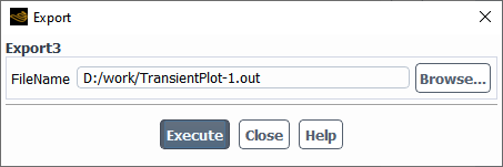
For the Filename, use the Browse... button or enter the name and location of the relevant report file(s) that you want to export.
Data from any number of report files can be added to and removed from a transient plot using the Report Files dialog, accessible from the relevant transient report property page.
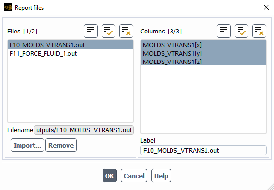
Use the Import... button to load report files (indicated in the Filenames field) into the Files column. Relevant data therein is listed in the Columns, with its default Label that can be changed accordingly. Use the Remove button to remove a selected file(s) from the report.