For heat conduction in a fixed solid region, Ansys Polyflow solves the energy equation in the following form:

(13–1)

where	= time derivative of the temperature
	= density
	= specific heat capacity
	= heat generated per unit volume by external sources
	= heat flux

Ansys Polyflow assumes that heat conduction is governed by Fourier’s law:

(13–2)

where is the thermal conductivity, which can be constant or temperature dependent. can also be constant or temperature dependent.

When solving steady problems in the absence of heat transport in the solid,

(13–3)

so the heat conduction model only requires the single parameter . For unsteady problems, you also need to supply and .

There are also situations where a motion is assigned to the solid body. Such is the case in processes like wire coating or extrusion of profiles with a metal insert which involve the motion of a rigid body at an assigned velocity. When such simulations are performed in a non-isothermal context, the heat transport originating from the assigned rigid body motion must be considered. From the point of view of the mathematics, a transport term is added to Equation 13–1 which becomes

(13–4)

In this term, the quantity denotes the (given) translation velocity of the rigid body. This requires additional parameters to be asked during the setup.

For nonisothermal flows, additional terms are included in the energy equation:

(13–5)

where	= Cauchy stress tensor
	= rate-of-deformation tensor

In Equation 13–5, the term represents the viscous dissipation, which can be important for high viscosity materials. The quantity represents a possible external heat source. Finally, is the material derivative of the temperature:

(13–6)

A heat flux condition can be imposed on external boundaries of the domain. Ansys Polyflow uses the following equation to compute the heat flux:

(13–7)

where is a temperature-independent heat flux and is the heat convection coefficient. The term allows the heat flux to be defined as a constant.

The second term stands for heat exchange by convection; is the temperature at the boundary and is the reference temperature for the convective heat exchange. The last term represents the heat exchange by radiation as given by the Stefan-Boltzmann law:

(13–8)

Here, is the coefficient of radiation, which is equal to the Stefan-Boltzmann constant in the case of black bodies (that is, 5.6704 10^-8 W/m²-K⁴). For non-black bodies, is equal to the product of the Boltzmann constant and an emissivity. Currently in Ansys Polyflow is assumed constant; the variation of emissivity with temperature is not available. is the reference temperature for the radiative heat exchange.

In its original formulation, the Stefan-Boltzmann law describes a relation between the heat flux and the absolute temperature. The temperature can also be specified relative to a nonzero reference temperature .

The Boussinesq approximation can be used instead of a constant density. This model treats density as a constant value in all solved equations, except for the buoyancy term in the momentum equation:

(13–9)

where is the (constant) density of the fluid, is a reference temperature, and is the thermal expansion coefficient. Equation 13–9 is obtained by using the Boussinesq approximation to eliminate from the buoyancy term. This approximation is accurate as long as changes in actual density are small.

A typical application of the Boussinesq approximation is a glass furnace model with natural-convection-induced vortices.

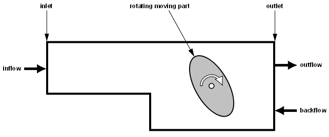
Special consideration must be given to boundaries that experience both incoming and outgoing flows as part of a nonisothermal simulation. Typically, such circumstances arise in outlets of the flow domain through which some fluid enters as backflow, although it is possible that you may observe an inlet section that has a mix of entering and exiting velocities. In such circumstances you must impose a temperature on the incoming flow; this is necessary because the temperature must be fixed at the start of every pathline that begins on the border of a flow domain in order to maintain the stability of the calculation.

Outlets may experience backflow as a result of rotating moving parts (such as the screws in extruders), especially if only a part of the full flow domain is simulated, for example, a few pitches of a full extruder. However, backflow can occur in cases that have no moving parts as well.

Figure 13.1: An Outlet with Backflow

The temperature is imposed on the incoming flow via a penalty formulation. The energy equation (Equation 13–5) for the nodes on the boundary is modified as follows:

(13–10)

where	= the penalty coefficient
	= the local normal velocity (positive if entering the flow domain)
	= the minimum normal velocity
	= the imposed temperature
	= the Heaviside step function

The Heaviside step function is assigned a value based on the values of the local and minimum normal velocities:

(13–11)

Note that no condition is imposed on the outgoing flow.