


To use the density-based solver you must first select the solver type, and determine if the simulation is steady-state or transient from the General Task Page (see Choosing the Solver). The density based solver settings are available mainly in two task pages: the Solution Methods Task Page and the Solution Controls Task Page.
In the Solution Methods task page, you can select the following:
Solution formulation type: Implicit or Explicit
Flux Scheme type: Roe-FDS, AUSM, or Low Diffusion Roe-FDS
Flow equation and model equation spatial discretization accuracy
For the steady-state solution method, you can select additional solution options to accelerate convergence
Pseudo time method (Implicit formulation only)
Convergence acceleration for stretched meshes
High-Speed Numerics
For more details, see Enabling High-Speed Numerics.
For the transient formulation you can select
first-order implicit
second-order implicit and for the explicit solver formulation, you can also select the explicit transient formulation
In the Solution Controls task page, you can select the following:
For the density-based explicit solver, you can specify the Courant number, FAS multigrid level, and Residual smoothing
For the density-based implicit solver, you can need to enter only the Courant number
For both solver methods, you can enter the under-relaxation factors associated with other equations solved with the flow equations, such as equations of the turbulence model
The above options can be found in the following sections:
For Ansys Fluent’s density-based solver, the main control over the time-stepping scheme is the Courant number (CFL). The time step size is proportional to the CFL, as defined in Equation 23–89 in the Theory Guide.
Linear stability theory determines a range of permissible values for the CFL (that is, the range of values for which a given numerical scheme will remain stable). When you specify a permissible CFL value, Ansys Fluent will compute an appropriate time step size using Equation 23–89 in the Theory Guide. In general, taking a larger time step size leads to faster convergence, so it is advantageous to set the CFL as large as possible (within the permissible range).
The stability limits of the density-based implicit and explicit formulations are significantly different. The explicit formulation has a more limited range and requires lower CFL settings than does the density-based implicit formulation. Appropriate choices of CFL for the two formulations are discussed below.
Linear stability analysis shows that the maximum allowable CFL for the multi-stage scheme used in the density-based explicit formulation will depend on the number of stages used and how often the dissipation and viscous terms are updated (see Changing the Multi-Stage Scheme). But in general, you can assume that the multi-stage scheme is stable for Courant numbers up to 2.5. This stability limit is often lower in practice because of nonlinearities in the governing equations.
The default CFL for the density-based explicit formulation is 1.0, but you may be able to increase it for some 2D problems. You should generally not use a value higher than 2.0.
If your solution is diverging, that is, if residuals are rising very rapidly, and your problem is properly set up and initialized, this is usually a good sign that the Courant number must be lowered. Depending on the severity of the startup conditions, you may need to decrease the CFL to a value as low as 0.1 to 0.5 to get started. Once the startup transients are reduced you can start increasing the Courant number again.
Linear stability theory shows that the density-based implicit formulation is unconditionally stable. However, as with the explicit formulation, nonlinearities in the governing equations will often limit stability.
The default CFL for the density-based implicit formulation is 5.0. It is often possible to increase the CFL to 10, 20, 100, or even higher, depending on the complexity of your problem. You may find that a lower CFL is required during startup (when changes in the solution are highly nonlinear), but it can be increased as the solution progresses.
The coupled AMG solver has the capability to detect divergence of the multigrid cycles within a given iteration. If this happens, it will automatically reduce the CFL and perform the iteration again, and a message will be printed to the screen. Five attempts are made to complete the iteration successfully. Upon successful completion of the current iteration the CFL is returned to its original value and the iteration procedure proceeds as required.
A CFL report definition will be automatically created for the density-based implicit steady solver. This report definition can be utilized to track the CFL when solution steering (Solution Steering) or divergence prevention (Preventing Divergence Using Local Under-Relaxation) is activated.
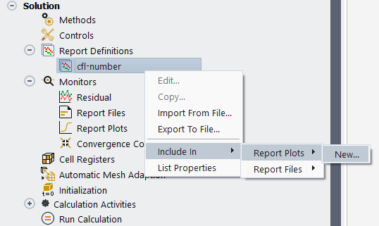
You can monitor the CFL by creating a plot and/or saving it to a file by right-clicking the report definition and selecting Include In → Report Plots/Report Files → New as shown in Figure 36.8: Creating CFL Report Plots and Files. For more details on creating Report Files or Report Plots, see Report Files and Report Plots.
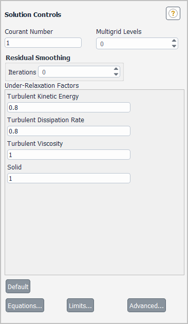
The Courant number is set in the Solution Controls Task Page (Figure 36.9: The Solution Controls Task Page for the Density-Based Explicit Formulation).
![]() Solution →
Solution → ![]() Controls
Controls
Enter the value for Courant Number.
When you select Explicit from the Formulation drop-down list in the Solution Methods Task Page, Ansys Fluent will automatically set the Courant Number to 1; when you select Implicit from the Formulation drop-down list, the Courant Number will be changed to 5 automatically.
The convective fluxes are selected from the Flux Type drop-down list in the Solution Methods task page.
![]() Solution →
Solution → ![]() Methods
Methods
You can select from the following when using the density-based solver:
Roe flux-difference splitting (Roe-FDS)
Roe-FDS splits the fluxes in a manner that is consistent with their corresponding flux method eigenvalues. It is the default and is recommended for most cases.
Advection Upstream Splitting Method (AUSM)
AUSM provides exact resolution of contact and shock discontinuities and it is less susceptible to Carbuncle phenomena.
Low diffusion Roe flux-difference splitting (Low Diffusion Roe-FDS)
Low Diffusion Roe-FDS is available when a Scale-Resolving Simulation (SRS) turbulence model is enabled along with the time-implicit formulation. It reduces the dissipation in turbulence calculations. This should be used only for subsonic flows.
Note: For cases that use an SRS turbulence model and/or include acoustic calculations, it is recommended that you use the
Roe-FDS with the Bounded Central Differencing (BCD) discretization scheme selected for
the flow equations, as this combination is more numerically robust than Low Diffusion Roe-FDS and just as
accurate. The BCD scheme alters the standard Roe-FDS scheme such that the diffusion is reduced. Note that if you are not using an
SRS turbulence model, to access the BCD scheme you will first need to enable the following text command:
solve/set/advanced/show-all-discretization-schemes.
When using the density-based solver with the implicit solution formulation in steady-state you can accelerate the convergence of your solution on highly-stretched and anisotropic meshes (like the one used when modeling external aerodynamic problems) by selecting the Convergence Acceleration For Stretched Meshes in the Solution Methods task page. For further information and theoretical background on this solution acceleration option, see Convergence Acceleration for Stretched Meshes in the Theory Guide. The Convergence Acceleration For Stretched Meshes option provides an optimum solution convergence of the implicit solution method.
To apply convergence acceleration for stretched meshes, perform the following:
Specify the solver options by selecting Density-Based and Steady in the General task page.
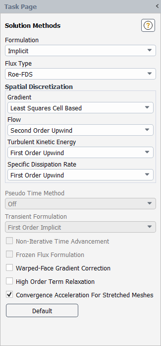
Select Implicit from the Formulation drop-down list and enable Convergence Acceleration For Stretched Meshes in the Solution Methods task page (Figure 36.10: The Solution Methods Task Page for the Density-Based Implicit Formulation).
Extra settings for CASM can be set using the following text command:
solve → set →
convergence-acceleration-for-stretched-meshes/
Enter yes in response to the Use convergence acceleration for stretched meshes
(CASM)? question. You will also be asked for a cut-off on the CFL value multiplier. By default this value is set to 100.
Typically, you do not need to adjust this value. But if convergence difficulties are encountered and reduction of the CFL value alone
does not help improve convergence, then it is advisable to reduce this CFL multiplier cut-off to a lower value (for example from 100
to 50, 20 or 10).
The use of CASM can typically give a much faster convergence over the standard solution method. In general, when using CASM, you do not need to specify a very large CFL value as you do with the standard solution method. A CFL value between 5 and 10 is typically used for converging most flow problems. When the Convergence Acceleration For Stretched Meshes option is selected, the solver will run when appropriate with a variable local CFL value proportional to the cell aspect ratios. Therefore, when the cell aspect ratio nears unity (typically far from walls), the local cell CFL value will be the same as the value that you supplied. However, as the cell is stretched and the cell aspect ratio increases (near walls), the local cell CFL value will be multiplied by the cell aspect ratio value. This is true until the cell stretching is beyond the multiplier cut-off value specified using the text command. The proportional change in CFL value on highly stretched cells helps accelerate the solution especially on highly packed and stretched meshes like the one used in modeling external flow problems.
When the cell aspect ratio is selected by default, the density-based implicit solver will operate with an explicit relaxation of
0.5 which can be adjusted by using the following text command:
solve/set/advanced/explicit-underrelaxation-value.
The convergence of the solution is mainly controlled by adjusting the CFL value. Therefore, if convergence problems are encountered, lowering the CFL value will help improve the convergence. Additional solution parameters to be adjusted for more conservative solution settings are:
lowering the density-based implicit solver explicit relaxation (
solve/set/advanced/explicit-underrelaxation-value)adjusting the CFL multiplier cut-off value to a lower value (
solve/set/convergence-acceleration-for-stretched-meshes/)
This solution convergence method is very aggressive. Therefore it is of paramount importance to start with a good initial guess especially if you start with second order spatial discretization. To get a good starting solution with the guess you provide, you are advised to use the full multi-grid initialization method (see Full Multigrid (FMG) Initialization).
Note: When the Convergence Acceleration For Stretched Meshes option is enabled, the Pseudo Time Method is turned off and is unavailable. You can either use Convergence Acceleration For Stretched Meshes or a Pseudo Time Method. These two cannot be used at the same time. Both methods help in obtaining faster convergence on anisotropic meshes. But one method requires that you enter a CFL value, while the other requires that you enter a pseudo time step value to march the solution to convergence. It is up to you to select the method with which you are most comfortable.
Convergence Acceleration For Stretched Meshes shows an advantage over the standard solution method, particularly with stretched meshes with low Y+ values (near unity). The use of Convergence Acceleration For Stretched Meshes results in an alteration of the numerical dissipation of the selected flux scheme. This change may slightly impact the monitored loading level if compared with the solution obtained without the use of this option.
The density-based solver offers an enhanced implementation of the convergence-acceleration for stretched meshes (CASM). This alternative formulation is similar to the standard CASM, but employs a cell aspect ratio formula which improves robustness on very high aspect ratio meshes and is more sensitive to changing flow topologies. It is also independent of the initial solution field. The enhanced CASM formulation is engaged with the following text command:
> solve/set/convergence-acceleration-for-stretched-meshes
Use convergence acceleration for stretched meshes (CASM)? [yes] no
Use enhanced CASM formulation? [yes] yes
Engaging enhanced CASM with explicit-relaxation factor: 0.75
Enter CASM cut-off multiplier : [100] 100
.
-------------------------------------------------------------------------------
 Convergence Acceleration for Stretched Meshes (CASM) has been selected.
 - The use of FMG initialization is highly recommended to provide good initial
   solution field before the start of calculations with CASM option.
 - Maximum benefit of CASM option is realized when local flow is aligned
   with mesh stretching.
------------------------------------------------------------------------------
Note that you must respond no to the first prompt and yes to the second prompt to
engage the enhanced CASM.
The enhanced CASM formulation uses an explicit under-relaxation of 0.75 by default.
When using the density-based solver, built-in customized numeric settings are available that can help to stabilize and accelerate the convergence for high-speed flows, see High Speed Numerics.
It is a sign of local divergence when the temperature and/or pressure for individual cells approaches the minimum and/or maximum
limits (set in the Solution Limits Dialog Box), and this can precede the divergence of the global solution. If either
of these quantities is being reset to a limiting value repeatedly (as indicated by the appropriate warning messages in the console),
you should check the dimensions, boundary conditions, and properties to be sure that the problem is set up correctly, and try to
determine the cause; you can create a field variable cell register to mark and display cells have a value equal to the limit (refer to
Field Variable for more information). If the setup appears appropriate but the density-based
solver still diverges, it is recommended that you use divergence prevention, which has been shown to be helpful for challenging cases
(such as those that undergo shocks or experience difficulties related to species calculations). With this option, Fluent will
identify the locally diverging cells and automatically apply a treatment to them that freezes the pressure and/or temperature values
(that is, sets the under-relaxation factor—which is similar to  in Equation 23–65 in the Fluent Theory Guide —to 0) and applies
under-relaxation to the other variables. To enable divergence prevention, use the following text command:
in Equation 23–65 in the Fluent Theory Guide —to 0) and applies
under-relaxation to the other variables. To enable divergence prevention, use the following text command:
solve → set → divergence-prevention
→ enable?
When prompted, enter yes, and then define the under-relaxation factor for the other variables: the
default value of 0.1 is recommended, though if this fails to prevent divergence you can try increasing this under-relaxation by
reducing the factor to 0.
Note: When you decide to enable divergence prevention, note the following: if the warning messages indicate that only a small percentage of cells are approaching the temperature and/or pressure limits, then you can just continue the calculation; if the percentage of cells is a higher value, it is recommended that you restart the calculation from initialization.
To improve the convergence to steady-state for some flow cases when using the density-based implicit solver you can specify the explicit relaxation using the following text command:
solve → set → advanced →
explicit-underrelaxation-value
Enter a value between 0 and 1.
For more information about explicit relaxation, see Under-Relaxation of Variables in the Theory Guide.
As discussed in Multigrid Method in the Theory Guide, FAS multigrid is an optional component of the density-based explicit formulation, while AMG multigrid is always on, by default for the density-based implicit formulation. Since nearly all density-based explicit calculations will benefit from the use of the FAS multigrid convergence accelerator, you should generally set a nonzero number of coarse grid levels before beginning the calculation. For most problems, this will be the only FAS multigrid parameter you will need to set. Should you encounter convergence difficulties, consider applying one of the methods discussed in Setting FAS Multigrid Parameters.
Important: Note that you cannot use FAS multigrid with explicit time stepping (described in Temporal Discretization in the Theory Guide) because the coarse grid corrections will destroy the time accuracy of the fine grid solution.
As discussed in Full-Approximation Storage (FAS) Multigrid in the Theory Guide, FAS multigrid solves on successively coarser grids and then transfers corrections to the solution back up to the original fine grid, thereby increasing the propagation speed of the solution and speeding convergence. The most basic way you can control the multigrid solver is by specifying the number of coarse grid levels to be used.
As explained in Full-Approximation Storage (FAS) Multigrid in the Theory Guide, the coarse grid levels are formed by agglomerating a group of adjacent “fine” cells into a single “coarse” cell. The optimal number of grid levels is therefore problem-dependent. For most problems, you can start out with 4 or 5 levels. For large 3D problems, you may want to add more levels (although memory restrictions may prevent you from using more levels, since each coarse grid level requires additional memory). If you believe that multigrid is causing convergence trouble, you can decrease the number of levels.
If Ansys Fluent reaches a coarse grid with one cell before creating as many levels as you requested, it will simply stop there. That is, if you request 5 levels, and level 4 has only 1 cell, Ansys Fluent will create only 4 levels, since levels 4 and 5 would be the same.
To specify the number of grid levels you want, set the number of Multigrid Levels in the Solution Controls Task Page (Figure 36.9: The Solution Controls Task Page for the Density-Based Explicit Formulation).
![]() Solution →
Solution → ![]() Controls
Controls
You can also set the Max Coarse Levels under FAS Multigrid Controls in the Multigrid tab in the Advanced Solution Controls Dialog Box.
Changing the number of coarse grid levels in the Solution Controls task page will automatically update the number shown in the Multigrid tab in the Advanced Solution Controls Dialog Box.
Coarse grid levels are created when you first begin iterating. If you want to check how many cells are in each level, request one iteration and then click Info and select Size in the Domain ribbon tab (Mesh group box) (as described in Mesh Size) to list the size of each grid level. If you are satisfied, you can continue the calculation; if not, you can change the number of coarse grid levels and check again.
For most problems, you will not need to modify any additional multigrid parameters once you have settled on an appropriate number of coarse grid levels. You can simply continue your calculation until convergence.
In the density-based explicit formulation, implicit residual smoothing (or averaging) is a technique that can be used to reduce the time step size restriction of the solver, thereby allowing the Courant number to be increased. The implicit smoothing is implemented with an iterative Jacobi method, as described in Implicit Residual Smoothing in the Theory Guide.
![]() Solution →
Solution → ![]() Controls
Controls
By default, the number of Iterations for Residual Smoothing is set to zero, indicating that residual smoothing is disabled. If you increase the Iterations counter to 1 or more, you can enter the Smoothing Factor. A smoothing factor of 0.5 with 2 passes of the Jacobi smoother is usually adequate to allow the Courant number to be doubled.