


Ansys Fluent provides several options for definition of the fluid viscosity:
constant viscosity
temperature-dependent and/or composition-dependent viscosity
kinetic theory
non-Newtonian viscosity
user-defined function
Each of these input options and the governing physical models are detailed in this section. (User-defined functions are described in the Fluent Customization Manual). In all cases, define the Viscosity in the Create/Edit Materials Dialog Box.
![]() Setup →
Setup → ![]() Materials
Materials
Viscosities are input as dynamic viscosity ( ) in units of kg/m-s
in SI units or
) in units of kg/m-s
in SI units or  /ft-s in British units. Ansys Fluent does not ask
for input of the kinematic viscosity (
/ft-s in British units. Ansys Fluent does not ask
for input of the kinematic viscosity ( ).
).
For additional information, see the following sections:
If you want to define the viscosity of your fluid as a constant, select constant in the Viscosity drop-down list in the Create/Edit Materials Dialog Box, and enter the value of viscosity for the fluid.
For the default fluid (air), the viscosity is  kg/m-s.
If you are modeling a problem that involves heat transfer, you can define the viscosity as a function of temperature. Five types of functions are available.


Important: The power law described here is different from the non-Newtonian power law described in Viscosity for Non-Newtonian Fluids.
For one of the first three, select piecewise-linear, piecewise-polynomial, polynomial in the Viscosity drop-down list and then enter
the data pairs ( ), ranges and coefficients, or coefficients
that describe these functions Defining Properties Using Temperature-Dependent Functions. For Sutherland’s
law or the power law, choose sutherland or power-law respectively in the drop-down list and
enter the parameters.
), ranges and coefficients, or coefficients
that describe these functions Defining Properties Using Temperature-Dependent Functions. For Sutherland’s
law or the power law, choose sutherland or power-law respectively in the drop-down list and
enter the parameters.
Sutherland’s viscosity law resulted from a kinetic theory by Sutherland (1893) using an idealized intermolecular-force potential. The formula is specified using two or three coefficients.
Sutherland’s law with two coefficients has the form
 | (8–24) |
| where, | |
 = the viscosity in kg/m-s = the viscosity in kg/m-s | |
 = the static temperature
in K = the static temperature
in K | |
 and and  = the coefficients = the coefficients |
For air at moderate temperatures and pressures,  kg/m-s-
 , and
, and  K.
K.
Sutherland’s law with three coefficients has the form
 | (8–25) |
| where, | |
 = the viscosity in kg/m-s = the viscosity in kg/m-s | |
 = the static temperature
in K = the static temperature
in K | |
 = reference
value in kg/m-s = reference
value in kg/m-s | |
 = reference
temperature in K = reference
temperature in K | |
 = an effective temperature in K (Sutherland constant) = an effective temperature in K (Sutherland constant) |
For air at moderate temperatures and pressures,  kg/m-s,
  =
273.11 K, and
=
273.11 K, and  = 110.56 K.
To use Sutherland’s law, choose sutherland in the drop-down list to the right of Viscosity. The Sutherland Law Dialog Box will open, and you can enter the coefficients as follows:
Select the Two Coefficient Method or the Three Coefficient Method.
Important: Use SI units if you choose the two-coefficient method.
For the Two Coefficient Method, set C1 and C2. For the Three Coefficient Method, set the Reference Viscosity
 , the Reference Temperature
  ,
and the Effective Temperature
,
and the Effective Temperature  .
.To visualize your profile, ensure the correct Primary Independent Variable is selected from the drop-down list, and enter a value for the Min and Max.
Another common approximation for the viscosity of dilute gases is the power-law form. For dilute gases at moderate temperatures, this form is considered to be slightly less accurate than Sutherland’s law.
A power-law viscosity law with two coefficients has the form
 | (8–26) |
| where, | |
 = the viscosity in
kg/m-s = the viscosity in
kg/m-s | |
 = the static temperature in K = the static temperature in K | |
 = a dimensional coefficient = a dimensional coefficient |
For air at moderate temperatures and pressures,  , and
, and  .
.
A power-law viscosity law with three coefficients has the form
 | (8–27) |
| where, | |
 = the viscosity in
kg/m-s = the viscosity in
kg/m-s | |
 = the static temperature in K = the static temperature in K | |
 = a reference value in K = a reference value in K | |
 = a reference value in kg/m-s = a reference value in kg/m-s |
For air at moderate temperatures and pressures,  kg/m-s,
  K, and
  .
.
Important: The non-Newtonian power law for viscosity is described in Viscosity for Non-Newtonian Fluids.
To use the power law, choose power-law in the drop-down list to the right of Viscosity. The Power Law Dialog Box will open, and you can enter the coefficients as follows:
Select the Two Coefficient Method or the Three Coefficient Method.
Important: Note that you must use SI units if you choose the two-coefficient method.
For the Two Coefficient Method, set B and the Temperature Exponent
 . For the Three Coefficient Method, set the Reference Viscosity
  , the Reference Temperature
  , and the Temperature Exponent
  .
.To visualize your profile, ensure the correct Primary Independent Variable is selected from the drop-down list, and enter a value for the Min and Max.
If you are using the ideal gas law (as described in Density), you have the option to define the fluid viscosity using kinetic theory as
 | (8–28) |
| where, | |
 is in units of kg/m-s, is in units of kg/m-s, | |
 is in units of Kelvin is in units of Kelvin | |
 is in units of Angstroms is in units of Angstroms | |

| |
 is the molecular weight is the molecular weight |
where
 | (8–29) |
The Lennard-Jones parameters,  and
and  , are inputs
to the kinetic theory calculation that you supply by selecting kinetic-theory from the drop-down list to the right
of Viscosity in the Create/Edit Materials Dialog Box. The solver will use these
kinetic theory inputs in Equation 8–28 to compute
the fluid viscosity. See Kinetic Theory Parameters for details about these inputs.
, are inputs
to the kinetic theory calculation that you supply by selecting kinetic-theory from the drop-down list to the right
of Viscosity in the Create/Edit Materials Dialog Box. The solver will use these
kinetic theory inputs in Equation 8–28 to compute
the fluid viscosity. See Kinetic Theory Parameters for details about these inputs.
When simulating hypersonic flows using the default one-temperature approach, Fluent offers Gupta curve fits that are applicable for air mixtures with temperatures up to 30 000 K. For details, see Modeling Transport Properties Using Gupta Curve Fits .
If you are modeling a flow that includes more than one chemical species (multicomponent flow), you have the option to define a composition-dependent viscosity. (Note that you can also define the viscosity of the mixture as a constant value or a function of temperature.)
To define a composition-dependent viscosity for a mixture, follow these steps:
For the mixture material, choose mass-weighted-mixing-law or, if you are using the ideal gas law for density, ideal-gas-mixing-law in the drop-down list to the right of Viscosity. If you have a user-defined function that you want to use to model the viscosity, you can choose either the user-defined method or the user-defined-mixing-law method for the mixture material in the drop-down list.
Click .
Define the viscosity for each of the fluid materials that make up the mixture. You may define constant or (if applicable) temperature-dependent viscosities for the individual species. You may also use kinetic theory for the individual viscosities, or specify a non-Newtonian viscosity, if applicable.
If you selected user-defined-mixing-law, define the viscosity for each of the fluid materials that make up the mixture. You may define constant, or (if applicable) temperature-dependent viscosities, or user-defined viscosities for the individual species. More information on defining properties with user-defined functions can be found in the Fluent Customization Manual.
The only difference between the user-defined-mixing-law and the user-defined option for specifying density, viscosity and thermal conductivity of mixture materials, is that with the user-defined-mixing-law option, the individual properties of the species materials can also be specified. (Note that only the constant, the polynomial methods and the user-defined methods are available.)
If you are using the ideal gas law, the solver will compute the mixture viscosity based on kinetic theory as
 | (8–30) |
where
 | (8–31) |
and  is the mole fraction of species
  .
.
For non-ideal gas mixtures, the mixture viscosity is computed based on a simple mass fraction average of the pure species viscosities:
 | (8–32) |
For incompressible Newtonian fluids, the shear stress is proportional
to the rate-of-deformation tensor  :
:
 | (8–33) |
where  is defined by
 | (8–34) |
and  is the viscosity, which is independent
of
is the viscosity, which is independent
of  .
.
For some non-Newtonian fluids, the shear stress can similarly
be written in terms of a non-Newtonian viscosity  :
:
 | (8–35) |
In general,  is a function of all three invariants of
the rate-of-deformation tensor
is a function of all three invariants of
the rate-of-deformation tensor  . However, in the non-Newtonian models available
in Ansys Fluent,
. However, in the non-Newtonian models available
in Ansys Fluent,  is considered to be a function of the shear
rate
is considered to be a function of the shear
rate  only.
only.  is related to the second invariant of
  and is defined as
 | (8–36) |
If the flow is non-isothermal, then the temperature dependence on the viscosity can be included along with the shear rate dependence. In this case, the total viscosity consists of two parts and is calculated as
 | (8–37) |
where H(T) is the temperature dependence, known as the Arrhenius law.
 | (8–38) |
where  is the ratio of the activation energy to
the thermodynamic constant and
is the ratio of the activation energy to
the thermodynamic constant and  is a reference temperature
for which H(T) = 1.
is a reference temperature
for which H(T) = 1.  , which is
the temperature shift, is set to 0 by default, and corresponds to
the lowest temperature that is thermodynamically acceptable. Therefore
, which is
the temperature shift, is set to 0 by default, and corresponds to
the lowest temperature that is thermodynamically acceptable. Therefore  and
and  are absolute temperatures. Temperature dependence
is only included when the energy equation is enabled. Set the parameter
are absolute temperatures. Temperature dependence
is only included when the energy equation is enabled. Set the parameter  to 0 when you want
temperature dependence to be ignored, even when the energy equation
is solved.
to 0 when you want
temperature dependence to be ignored, even when the energy equation
is solved.
Ansys Fluent provides four options for modeling non-Newtonian flows:
power law
Carreau model for pseudo-plastics
Cross model
Herschel-Bulkley model for Bingham plastics
Important:
Note that the models listed above are not available when modeling turbulent flow.
Note that the non-Newtonian power law described below is different from the power law described in Power-Law Viscosity Law.
Non-Newtonian model based on single fluid formulation is available for the mixture model and it is recommended that this should be attached to the primary phase.
Appropriate values for the input parameters for these models can be found in the literature (for example, [160]).
If you choose non-newtonian-power-law in the drop-down list to the right of Viscosity, non-Newtonian flow will be modeled according to the following power law for the non-Newtonian viscosity:
 | (8–39) |
where  and
and  are input parameters.
  is a measure of the average viscosity
of the fluid (the consistency index);
is a measure of the average viscosity
of the fluid (the consistency index);  is a measure of the deviation
of the fluid from Newtonian (the power-law index). The value of
is a measure of the deviation
of the fluid from Newtonian (the power-law index). The value of  determines the class of
the fluid:
determines the class of
the fluid:
 → Newtonian
fluid → Newtonian
fluid | |
 → shear-thickening (dilatant fluids) → shear-thickening (dilatant fluids) | |
 → shear-thinning (pseudo-plastics) → shear-thinning (pseudo-plastics) |
To use the non-Newtonian power law, choose non-newtonian-power-law in the drop-down list to the right of Viscosity. The Non-Newtonian Power Law Dialog Box will open,
and you can choose between Shear Rate Dependent and Shear Rate and Temperature Dependent. Enter
the Consistency Index  , Power-Law Index
  , Minimum and Maximum
Viscosity Limit, Reference Temperature
, Minimum and Maximum
Viscosity Limit, Reference Temperature  , and Activation Energy/R,
  , which is the ratio of the activation energy
to the thermodynamic constant.
, which is the ratio of the activation energy
to the thermodynamic constant.
The power law model described in Equation 8–39 results in a fluid viscosity that varies with shear rate. For  ,
,  , and for
  ,
,  , where
  and
and  are, respectively,
the upper and lower limiting values of the fluid viscosity.
are, respectively,
the upper and lower limiting values of the fluid viscosity.
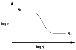
The Carreau model attempts to describe a wide range of fluids
by the establishment of a curve-fit to piece together functions for
both Newtonian and shear-thinning ( ) non-Newtonian laws. In the Carreau model,
the viscosity is
) non-Newtonian laws. In the Carreau model,
the viscosity is
 | (8–40) |
and the parameters  ,
,  ,
,  ,
,  , and
, and  are dependent
upon the fluid.
are dependent
upon the fluid.  is the time constant,
  is the power-law index (as
described above for the non-Newtonian power law),
is the power-law index (as
described above for the non-Newtonian power law),  and
and  are, respectively,
the zero- and infinite-shear viscosities,
are, respectively,
the zero- and infinite-shear viscosities,  is the reference
temperature, and
is the reference
temperature, and  is the ratio of the activation energy to
thermodynamic constant. Figure 8.19: Variation of Viscosity with Shear Rate According to the Carreau
Model shows
how viscosity is limited by
is the ratio of the activation energy to
thermodynamic constant. Figure 8.19: Variation of Viscosity with Shear Rate According to the Carreau
Model shows
how viscosity is limited by  and
and  at
low and high shear rates.
at
low and high shear rates.
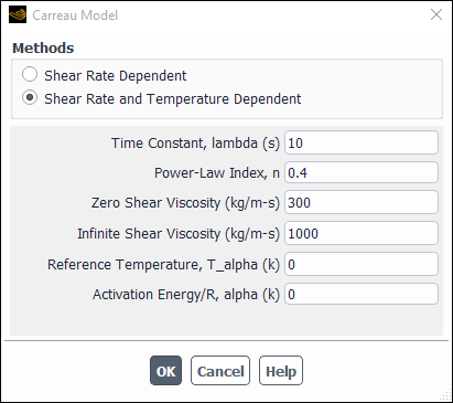
To use the Carreau model, choose carreau in the drop-down list to the right of Viscosity. The Carreau Model Dialog Box will open, and you can
choose between Shear Rate Dependent and Shear Rate and Temperature Dependent. Enter the Time Constant  , Power-Law Index
  , Reference Temperature
  , Zero Shear
Viscosity
, Zero Shear
Viscosity  , Infinite Shear Viscosity
  ,
and Activation Energy/R
,
and Activation Energy/R  .
.
The Cross model for viscosity is:
 | (8–41) |
| where, | |
 = zero-shear-rate
viscosity = zero-shear-rate
viscosity | |
 = natural time (that
is, inverse of the shear rate at which the fluid changes from Newtonian
to power-law behavior) = natural time (that
is, inverse of the shear rate at which the fluid changes from Newtonian
to power-law behavior) | |
 = power-law index = power-law index |
The Cross model is commonly used to describe the low-shear-rate behavior of the viscosity.
To use the Cross model, choose cross in
the drop-down list to the right of Viscosity. The Cross Model Dialog Box will open, and you can
choose between Shear Rate Dependent and Shear Rate and Temperature Dependent. Enter the Zero Shear Viscosity  , Time Constant
  , Power-Law
Index
, Power-Law
Index  , Reference Temperature
  ,
and Activation Energy/R,
,
and Activation Energy/R,  , which is the ratio of
the activation energy to the thermodynamic constant.
, which is the ratio of
the activation energy to the thermodynamic constant.
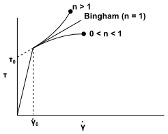
The power law model described above is valid for fluids for which the shear stress is zero when the strain rate is zero. Bingham plastics are characterized by a nonzero shear stress when the strain rate is zero.
 | (8–42) |
where  is the yield
stress:
is the yield
stress:
For
 , the material remains
rigid.
, the material remains
rigid.For
 , the material flows
as a power-law fluid.
, the material flows
as a power-law fluid.
The Herschel-Bulkley model combines the effects of Bingham and
power-law behavior in a fluid. For low strain rates ( ), the “rigid”
material acts like a very viscous fluid with viscosity
), the “rigid”
material acts like a very viscous fluid with viscosity  . As the strain rate increases and the yield stress
threshold,
. As the strain rate increases and the yield stress
threshold,  , is passed,
the fluid behavior is described by a power law.
, is passed,
the fluid behavior is described by a power law.
For 
 | (8–43) |
For 
 | (8–44) |
where  is the consistency index, and
  is the power-law index.
Figure 8.21: Variation of Shear Stress with Shear Rate According to the
Herschel-Bulkley Model shows how shear stress
( ) varies with shear rate (
 ) for the Herschel-Bulkley model.
If you choose the Herschel-Bulkley model for Bingham plastics, Equation 8–43 will be used to determine the fluid viscosity.
The Herschel-Bulkley model is commonly used to describe materials
such as concrete, mud, dough, and toothpaste, for which a constant
viscosity after a critical shear stress is a reasonable assumption.
In addition to the transition behavior between a flow and no-flow
regime, the Herschel-Bulkley model can also exhibit a shear-thinning
or shear-thickening behavior depending on the value of  .
.
To use the Herschel-Bulkley model, choose herschel-bulkley in the drop-down list to the right of Viscosity. The Herschel-Bulkley Dialog Box will open, and you
can choose between Shear Rate Dependent and Shear Rate and Temperature Dependent. Enter the Consistency Index  , Power-Law Index
  , Yield Stress
Threshold
, Yield Stress
Threshold  , Critical Shear Rate
  , Reference Temperature
  , and the ratio of the
activation energy to thermodynamic constant
, and the ratio of the
activation energy to thermodynamic constant  , Activation Energy/R.