


As mentioned earlier, in most cases the multigrid solver will not require any special attention from you. If, however, you have convergence difficulties or you want to minimize the overall solution time by using more aggressive settings, you can monitor the multigrid solver and modify the parameters to improve its performance. (The instructions below assume that you have already begun calculations, since there is no need to monitor the solver if you do not fit into one of the two categories above.)
To determine whether your convergence difficulties can be alleviated by modifying the multigrid settings, you will check if the requested residual reduction is obtained on each grid level. To minimize solution time, you will check to see if switching to a more powerful cycle will result in overall reduction of work by the solver.
By default, the flexible cycle is used for all equations except pressure correction, which uses a V cycle. Typically, for a flexible cycle only a few (5–10) relaxations will be performed at the finest level and no coarse levels will be visited. In some cases one or two coarse levels may be visited. If the maximum number of fine level relaxations is not sufficient, you may want to increase the maximum number (as described in Flexible Cycle Parameters) or switch to a V cycle (as described in Specifying the Multigrid Cycle Type).
In the pressure-based segregated algorithm, the pressure correction uses a V cycle by default. If the maximum number of cycles (30 by default) is not sufficient, you can switch to a W cycle (using the Multigrid tab in the Advanced Solution Controls Dialog Box, as described in Specifying the Multigrid Cycle Type). Note that efficiency may deteriorate with a W cycle.
You can try increasing the maximum number of cycles by increasing the value of Max Cycles in the Multigrid tab, under Fixed Cycle Parameters.
In the pressure-based coupled algorithm and the density-based implicit formulation, there is no pressure correction. Instead, there is a flow correction, which by default uses the F cycle. The density-based explicit formulation uses the V cycle as the default flow correction.
![]() Solution →
Solution → ![]() Controls →
Advanced...
Controls →
Advanced...
For additional information, see the following sections:
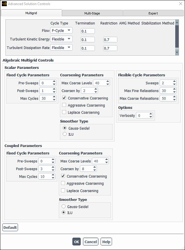
By default, the V cycle is used for the pressure equation in the pressure-based segregated algorithm and the flexible cycle is used for all other equations with the exception that the F cycle is used for energy. In the pressure-based coupled algorithm, the F cycle is the default for the coupled flow equations and for the energy equation. All other scalar equations use the flexible cycle by default. In the density-based implicit formulation, the F cycle is default for the flow correction. The V cycle is default for the flow correction in the density-based explicit formulation. For both density-based formulations the flexible cycle is used for the scalar equations. (See Multigrid Cycles in the Theory Guide for a description of these cycles.) To change the cycle type for an equation, you will use the top portion of the Multigrid tab in the Advanced Solution Controls Dialog Box (Figure 36.11: The Multigrid Tab).
For each equation, you can choose Flexible, V-Cycle, W-Cycle, or F-Cycle in the adjacent drop-down list.
When you use the flexible cycle for an equation, you can control the multigrid performance by modifying the Termination and/or Restriction criteria for that equation at the top of the Multigrid tab in the Advanced Solution Controls Dialog Box (Figure 36.11: The Multigrid Tab).
![]() Solution →
Solution → ![]() Controls →
Advanced...
Controls →
Advanced...
The Restriction criterion is the residual reduction tolerance,  in Equation 23–131 in the Theory Guide. This parameter dictates when a coarser grid level must be visited (due to insufficient
improvement in the solution on the current level). With a larger value of
in Equation 23–131 in the Theory Guide. This parameter dictates when a coarser grid level must be visited (due to insufficient
improvement in the solution on the current level). With a larger value of  , coarse levels will be visited less often (and vice versa). The Termination criterion,
 in Equation 23–132 in the Theory Guide, governs when the solver should return to a finer grid level (that is, when the residuals
have improved sufficiently on the current level).
in Equation 23–132 in the Theory Guide, governs when the solver should return to a finer grid level (that is, when the residuals
have improved sufficiently on the current level).
For the V, W, or F cycle, the Termination criterion determines whether or not another cycle should be performed on the finest (original) level. If the current residual on the finest level does not satisfy Equation 23–132 in the Theory Guide, and the maximum number of cycles has not been performed, Ansys Fluent will perform another multigrid cycle. (The Restriction parameter is not used by the V, W, and F cycles.)
The AMG solver [171] builds coarse levels by grouping fine level cells to make coarse level cells, and uses piecewise constant interpolation.
In the Multigrid tab (Figure 36.11: The Multigrid Tab), you can choose another stabilization method rather than the AMG solver if you are using a fixed-type cycle (F, V, or W cycle); this is available for all equations except the flow correction for the density-based solver. If desired, you can choose the bi-conjugate gradient stabilized method [16] (BCGSTAB) option, the recursive projection method [142] (RPM), or the generalized minimal residual method [134] (GMRES) in order to improve the convergence of the linear solver. BCGSTAB and GMRES can be preconditioned, and all these methods can provide more stability and robustness than the AMG solver.
Ansys Fluent usually builds diagonally dominant matrices for the linear solver. However, this is not always possible. A linear system with highly dominant off-diagonal coefficients may occur during discretization of complex physical models such as multiphase cavitation. Using a stabilization method in such cases can be helpful. In addition, the AMG convergence in parallel can be improved using the BCGSTAB or GMRES option with AMG. It is recommended that you attempt a solution first with BCGSTAB; the GMRES is usually more robust and more likely to converge, but it is more demanding in terms of memory usage and solver time.
If you are using the pressure-based segregated solver and the flow is incompressible, an additional stabilization method for the algebraic multigrid solver will appear in the Stabilization Method drop-down list. This is the conjugate gradient method, or CG [16] and will be available only for the pressure equation. This method is typically used in conjunction with an AMG preconditioner (any available AMG method). The CG formulation requires a symmetric system matrix. Such matrices result from the finite volume discretization of steady or transient elliptic operators, such as the pressure correction equation in the incompressible case. The CG method provides a useful alternative to BCGSTAB, RPM, and GMRES, since it reduces the memory requirements and the number of floating point operations, especially when compared to BCGSTAB. In addition, in transient pressure-based segregated solvers, as typically used in LES and/or NITA simulations, the solution of the pressure correction equation constitutes a significant share of the overall computational effort.
Note that when divergence is detected for the AMG solver, the BCGSTAB method and/or the CG method, then an alternate method will be used for an iteration as a fallback, and you will be informed in the console that an equation is being stabilized to enhance linear solver robustness. If you see such console messages repeatedly for flow-related equations, it is an indication that you need to revise the settings in the Solution Methods task page and/or the Algebraic Multigrid Controls group box of the Advanced Solution Controls dialog box.
There are several additional parameters that control the algebraic multigrid solver, but there will usually be no need to modify them. These additional scalar and coupled parameters are all contained in the Multigrid tab in the Advanced Solution Controls Dialog Box (Figure 36.11: The Multigrid Tab).
![]() Solution →
Solution → ![]() Controls →
Advanced...
Controls →
Advanced...
Important: When using the density-based explicit formulation or the pressure-based solver with any of the segregated algorithms, described in Pressure-Velocity Coupling in the Theory Guide and Choosing the Pressure-Velocity Coupling Method, only Scalar Parameters are set in the Multigrid tab. If you use the density-based implicit or the pressure-based coupled algorithm, described in Coupled Algorithm in the Theory Guide, then you can set the Coupled Parameters.
For the fixed (V, W, and F) multigrid cycles, you can control the number of pre- and post-relaxations (
 and
and  in Multigrid Cycles in the Theory Guide). Pre-Sweeps sets the number of relaxations to perform before moving
to a coarser level. Post-Sweeps sets the number to be performed after coarser level corrections have been
applied. Normally, under Scalar Parameters, one post-relaxation is performed and no pre-relaxations are done
(that is,
in Multigrid Cycles in the Theory Guide). Pre-Sweeps sets the number of relaxations to perform before moving
to a coarser level. Post-Sweeps sets the number to be performed after coarser level corrections have been
applied. Normally, under Scalar Parameters, one post-relaxation is performed and no pre-relaxations are done
(that is,  and
and  ), but in rare cases, you may need to increase the value of
  to 1 or 2. Under Coupled Parameters, three post-relaxations are performed by default with
no pre-relaxations. If you are using the pressure-based coupled solver for a steady simulation with a pseudo time method selected,
three post-relaxations are performed under Scalar Parameters also.
to 1 or 2. Under Coupled Parameters, three post-relaxations are performed by default with
no pre-relaxations. If you are using the pressure-based coupled solver for a steady simulation with a pseudo time method selected,
three post-relaxations are performed under Scalar Parameters also.
Important:
If you are using AMG with V-cycle to solve an energy equation with a solid conduction model presented with anisotropic or very high conductivity coefficient, there is a possibility of divergence with a default post-relaxation sweep of
 . In such cases you should increase the post-relaxation sweep (to say
  ) in the AMG section for better convergence when using the pressure-based segregated algorithms.
It is recommended that you use the Fixed F-cycle for the energy equation when running parallel Ansys Fluent.
For all multigrid cycle types, you can control the maximum number of coarse levels (Max Coarse Levels under Scalar or Coupled Parameters) that will be built by the multigrid solver.
Sets of coarser simultaneous equations are built until the maximum number of levels has been created, or the coarsest level has only 3 equations. Each level has about half as many unknowns as the previous level, so coarsening until there are only a few cells left will require about as much total coarse-level coefficient storage as was required on the fine mesh. Reducing the maximum coarse levels will reduce the memory requirements, but may require more iterations to achieve a converged solution. Setting Max Coarse Levels to 0 turns off the algebraic multigrid solver.
Another coarsening parameter you can control is the increase in coarseness on successive levels. The Coarsen by parameter specifies the number of fine grid cells that will be grouped together to create a coarse grid cell. The algorithm groups each cell with its strongest neighbor, then groups the cell and its strongest neighbor with the neighbor’s strongest neighbor, continuing until the desired coarsening is achieved. Typical values for the scalar parameters are in the range from 2 to 10, with the default value of 2 for the Gauss-Seidel smoother giving the best performance, but also the greatest memory use. For coupled parameters and scalar parameters when using the pressure-based coupled solver with the pseudo method option enabled, the default values of 4 (for 2D) and 8 (for 3D) for the ILU smoother give the best performance. You should not adjust this parameter unless you need to reduce the memory required to run a problem.
Important: Depending on the smoother type, Gauss-Seidel or ILU, the Coarsen by and Post-Sweeps settings should be changed as follows when selecting the non-default smoother type:
- ILU
: Post-Sweeps =3 and Coarsen by = 8
- Gauss-Seidel
: Post-Sweeps =1 and Coarsen by = 2
For the scalar and coupled equations, you have the following AMG coarsening options. Note that these can be used singly or in combination with each other.
Conservative Coarsening
This option is enabled by default, and improves convergence for difficult problems by tuning multigrid coarsening based on coefficient strengths and, in parallel computations, the partitioning.
Aggressive Coarsening
This option specifies the use of a version of the AMG solver that is optimized for higher, more aggressive coarsening rates. It is recommended if the AMG solver diverges with the default settings, and is more likely to be beneficial in the following cases:
if the corresponding Coarsen by field is set to a value greater than 2 (which is the case by default if you are using the density-based implicit or the pressure-based coupled scheme)
if you are using higher core counts
Laplace Coarsening
This option is disabled by default, so that a cell’s strongest neighbor is identified based on the magnitude of its interaction with the cell in question. Enabling it specifies that Laplace coefficients are used to evaluate neighbor strength when grouping cells for coarsening. This may improve stability in some cases because the coarser levels will not change as the solution evolves. It may also reduce computation time, particularly at high core counts, because the coarse levels don’t need to be recreated every iteration.
Two smoother types are available for scalar and coupled parameters. Gauss-Seidel is the simplest smoother type and is recommended when using the pressure-based segregated algorithm. ILU is more CPU intensive, but has better smoothing properties for block-coupled systems such as the pressure-based coupled solver and the density-based implicit formulation. The default scalar Smoother Type is Gauss-Seidel, while the coupled Smoother Type is ILU. The ILU smoother is also used for scalar equations when using the coupled solver with a pseudo time method selected. For more information about the two smoother types, see The Coupled and Scalar AMG Solvers in the Theory Guide.
To change the maximum number of relaxations, increase or decrease the value of Max Fine Relaxations or Max Coarse Relaxations in the Multigrid tab in the Advanced Solution Controls Dialog Box (Figure 36.11: The Multigrid Tab) under Flexible Cycle Parameters.
![]() Solution →
Solution → ![]() Controls →
Advanced...
Controls →
Advanced...
The steps for monitoring the solver are as follows:
Set multigrid Verbosity to 1 or 2 in the Multigrid tab in the Advanced Solution Controls Dialog Box.
 Solution →
  Controls →
Advanced...
Controls →
Advanced...Request a single iteration using the Run Calculation Task Page.
Solution → Run Calculation
If you set the verbosity to 2, the information printed in the Ansys Fluent console for each equation will include the following:
equation name
equation tolerance (computed by the solver using a normalization of the source vector)
residual value after each fixed multigrid cycle or fine relaxation for the flexible cycle
number of equations in each multigrid level, with the zeroth level being the original (finest-level) system of equations
Note that the residual printed at cycle or relaxation 0 is the initial residual before any multigrid cycles are performed.
When verbosity is set to 1, only the equation name, tolerance, and residuals are printed.
A portion of a sample printout is shown below:
 pressure correction equation:
 tol. 1.2668e-05
  0 2.5336e+00
  1 4.9778e-01
  2 2.5863e-01
  3 1.9387e-01
  multigrid levels:
  0 918
  1 426
  2 205
  3  97
  4  45
  5  21
  6  10
  7  4
If you change the multigrid parameters, but you then want to return to Ansys Fluent’s default settings, you can click the button in the Multigrid tab. Ansys Fluent will change all settings to the defaults, and the button will become the Reset button. To get your settings back again, you can click the button.
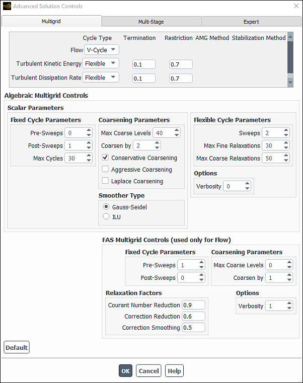
For most calculations, you will not need to modify any FAS multigrid parameters once you have set the number of coarse grid levels. If, however, you encounter convergence difficulties, you may consider the following suggested procedures.
Important: Recall that FAS multigrid is used only by the density-based explicit formulation.
Some problems may approach convergence steadily at first, but then the residuals will level off and the solution will “get stuck.” In some cases (for example, long thin ducts), this convergence trouble may be due to multigrid’s slow propagation of pressure information through the domain. In such cases, you should turn off multigrid by setting Multigrid Levels to 0 in the Solution Controls Task Page.
In some cases, you may find that your problem is converging, but at an extremely slow rate. Such problems can often benefit from a more aggressive form of multigrid, which will speed up the propagation of the solution corrections. For such problems, you can try the “industrial-strength” multigrid settings.
Important: These settings are very aggressive and assume that the solution information passed through the multigrid levels is somewhat accurate. For this reason, you should only attempt the procedure described here after you have performed enough iterations that the solution is off to a good start. Using “industrial-strength” multigrid too early in the calculation process—when the solution is far from correct—will not help convergence and may cause the calculation to become unstable, as very incorrect values are propagated quickly to the original grid. Note also that while these multigrid settings will usually reduce the total number of iterations required to reach convergence, they will greatly increase the computation time for each multigrid cycle. Thus the solver will be performing fewer but longer iterations.
The strategy employed is as follows:
Increase the number of iterations performed on each grid level before proceeding to a coarser level
Increase the number of iterations performed on each grid level after returning from a coarser level
Allow full correction transfer from one level to the next finer level, instead of transferring reduced values of the corrections
Do not smooth the interpolated corrections when they are transferred from a coarser grid to a finer grid
You can set all of the parameters for this strategy under FAS Multigrid Controls in the Multigrid tab in the Advanced Solution Controls Dialog Box (Figure 36.12: The Advanced Solution Controls Dialog Box) and then continue the calculation.
![]() Solution →
Solution → ![]() Controls →
Advanced...
Controls →
Advanced...
Increasing the number of iterations performed on each grid level before proceeding to a coarser level (the value of
 described in Multigrid Cycles in the Theory Guide) will improve the solution passed from each finer grid level to the next coarser grid
level. Try increasing the value of Pre-Sweeps (under FAS Multigrid Controls,
not under Algebraic Multigrid Controls) to 10.
described in Multigrid Cycles in the Theory Guide) will improve the solution passed from each finer grid level to the next coarser grid
level. Try increasing the value of Pre-Sweeps (under FAS Multigrid Controls,
not under Algebraic Multigrid Controls) to 10.
Increasing the number of iterations performed on each level after returning from a coarser level will improve the corrections passed from each coarser grid level to the next finer grid level. Errors introduced on the coarser grid levels can therefore be reduced before they are passed further up the grid hierarchy to the original grid. Try increasing the value of Post-Sweeps (under FAS Multigrid Controls, not under Algebraic Multigrid Controls) to 10.
By default, the full values of the multigrid corrections are not transferred from a coarser grid to a finer grid; only 60% of the value is transferred. This prevents large errors from transferring quickly up to the original grid and causing the calculation to become unstable. It also prevents a “good” solution from propagating quickly to the original grid. However, by increasing the Correction Reduction to 1, you can transfer the full values from coarser to finer grid levels, speeding the propagation of the solution and, usually, the convergence as well. The Species Correction Reduction sets the factor by which to reduce the magnitude of the species corrections to stabilize the multigrid calculation. This item appears only when species transport is being modeled.
When the corrections on a coarse grid are passed back to the next finer grid level, the values are, by default, interpolated and then smoothed. Disabling the smoothing so that the actual value in a coarse grid cell is assigned to the fine grid cells that make it up can also aid convergence. To disable smoothing, set the Correction Smoothing to 0. Large discontinuities between cells will be smoothed out implicitly as a result of the additional Post-Sweeps performed.
The Courant Number Reduction sets the factor by which to reduce the Courant number for coarse grid levels (that is, every level except the finest). Some reduction of the time step size (such as the default 0.9) is typically required because the stability limit cannot be determined as precisely on the irregularly shaped coarser grid cells.