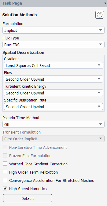
When using the density-based solver, built-in customized numeric settings are available that can help to stabilize and accelerate the convergence for high-speed flows. High-Speed Numerics (HSN) are enabled from the Solution Methods task page:

  → Solution → Solution → Methods...

Or by entering the following text command in the console: solve/set/high-speed-numerics/enable? yes

By default, the adaptive HSN mode will be selected. This formulation adjusts the numerics proportionally to the strength of the captured shockwave and is well suited for general shock-dominated problems. The adaptive mode is also advantageous for flows containing multiple shockwaves of different strengths, and possibly interacting with one another.

You can access more conservative high-speed numerics setting in the expert submenu if the default adaptive option is not providing the desired level of stabilization. However, in most situations, you do not need to access this submenu and the solution stability can be resolved with the default adaptive high-speed numerics and the adjustment of the CFL value.

solve/set/high-speed-numerics/expert

You will then be asked to enter a single digit (0 - 5) corresponding to a Mach number range that best characterizes the flow, as shown:

[      Mach < 0.7] Disabled = 0
[0.7 < Mach < 1.4] Transonic = 1
[1.4 < Mach < 2.5] Low-Supersonic = 2
[2.5 < Mach < 4.5] High-Supersonic = 3
[4.5 < Mach      ] Hypersonic = 4
[0.0 < Mach < Inf] Adaptive (Default) = 5

The range you select will determine the nature of the changes to the settings. For Mach numbers less than 0.7, HSN are not required and will not be applied; instead, the regular solver defaults and settings you have defined will be used. For Mach regimes 1 - 4, HSN with increasing levels of stabilization are used to achieve fast convergence, while maintaining a high level of solution accuracy. Choosing 5 recovers the adaptive mode, which is the default mode of operation suitable for the widest range of flows.

HSN are compatible with both the Roe-FDS and AUSM flux schemes. They can also be used effectively with the Convergence Acceleration For Stretched Meshes (CASM) option. Although HSN are available for transient simulations, they are often not required for cases in which the shock is traveling (such as a traveling shock front) or constantly moving (such as the shock for an oscillating transonic airfoil/wing). HSN can be used if the location of the shock changes initially but then stabilizes.

When HSN are enabled, a field variable is available to help display the shock front. It is made available with the following text command:

solve/set/high-speed-numerics/visualize-pressure-discontinuity-sensor? yes

The variable Pressure Discontinuity Sensor (in the Pressure... category) is a binary identifier based on whether a cell is in proximity to a pressure discontinuity (in which case the value = 1) or not (value = 0). Note that this field variable will display only the strongest part of the shock front and not necessarily the entire shock system; often the shock runs longer than indicated.