


This algorithm is referred to as an "algebraic" multigrid scheme because, as we shall see, the coarse level equations are generated without the use of any geometry or re-discretization on the coarse levels; a feature that makes AMG particularly attractive for use on unstructured meshes. The advantage being that no coarse meshes have to be constructed or stored, and no fluxes or source terms need to be evaluated on the coarse levels. This approach is in contrast with FAS (sometimes called "geometric") multigrid in which a hierarchy of meshes is required and the discretized equations are evaluated on every level. In theory, the advantage of FAS over AMG is that the former should perform better for non-linear problems since non-linearities in the system are carried down to the coarse levels through the re-discretization; when using AMG, once the system is linearized, non-linearities are not "felt" by the solver until the fine level operator is next updated.
The restriction and prolongation operators used here are based on the additive correction (AC) strategy described for structured meshes by Hutchinson and Raithby [265]. Inter-level transfer is accomplished by piecewise constant interpolation and prolongation. The defect in any coarse level cell is given by the sum of those from the fine level cells it contains, while fine level corrections are obtained by injection of coarse level values. In this manner the prolongation operator is given by the transpose of the restriction operator
 | (23–123) |
The restriction operator is defined by a coarsening or "grouping" of fine level cells into coarse level ones. In this process each fine level cell is grouped with one or more of its "strongest" neighbors, with a preference given to currently ungrouped neighbors. The algorithm attempts to collect cells into groups of fixed size, typically two or four, but any number can be specified.
By default, the “strongest” neighbor is evaluated as the neighbor
 of the current cell
  for which the coefficient
  is largest. For sets of coupled equations
  is a block matrix and the measure of its magnitude is simply taken to be the
magnitude of its first element. In addition, the set of coupled equations for a given cell are
treated together and not divided amongst different coarse cells. This results in the same
coarsening for each equation in the system.
is a block matrix and the measure of its magnitude is simply taken to be the
magnitude of its first element. In addition, the set of coupled equations for a given cell are
treated together and not divided amongst different coarse cells. This results in the same
coarsening for each equation in the system.
You have the option of enabling a conservative coarsening scheme that tunes the multigrid coarsening based on coefficient strengths and partitioning, as well as an aggressive coarsening scheme that is optimized for higher coarsening rates. Alternatively, you can enable Laplace coarsening so that Ansys Fluent uses Laplace coefficients as the strength factors in determining the coarsening. For details, refer to Coarsening Parameters in the Fluent User's Guide.
The coarse level operator  is constructed using a Galerkin
approach. Here we require that the defect associated with the corrected
fine level solution must vanish when transferred back to the coarse
level. Therefore we may write
is constructed using a Galerkin
approach. Here we require that the defect associated with the corrected
fine level solution must vanish when transferred back to the coarse
level. Therefore we may write
 | (23–124) |
Upon substituting Equation 23–116 and Equation 23–122 for  and
and  we have
 | (23–125) |
Now rearranging and using Equation 23–116 once again gives
 | (23–126) |
Comparison of Equation 23–126 with Equation 23–121 leads to the following expression for the coarse level operator:
 | (23–127) |
The construction of coarse level operators therefore reduces to a summation of diagonal and corresponding off-diagonal blocks for all fine level cells within a group to form the diagonal block of that group’s coarse cell.
The multigrid F cycle is essentially a combination of the V and W cycles described in The V and W Cycles.
Recall that the multigrid cycle is a recursive procedure. The procedure is expanded to the next coarsest grid level by performing a single multigrid cycle on the current level. Referring to Figure 23.9: V-Cycle Multigrid and Figure 23.10: W-Cycle Multigrid, this means replacing the square on the current level (representing a single cycle) with the procedure shown for the 0-1 level cycle (the second diagram in each figure). We see that a V cycle consists of:
 | (23–128) |
and a W cycle:
 | (23–129) |
An F cycle is formed by a W cycle followed by a V cycle:
 | (23–130) |
As expected, the F cycle requires more computation than the V cycle, but less than the W cycle. However, its convergence properties turn out to be better than the V cycle and roughly equivalent to the W cycle. The F cycle is the default AMG cycle type for the coupled equation set and for the scalar energy equation.
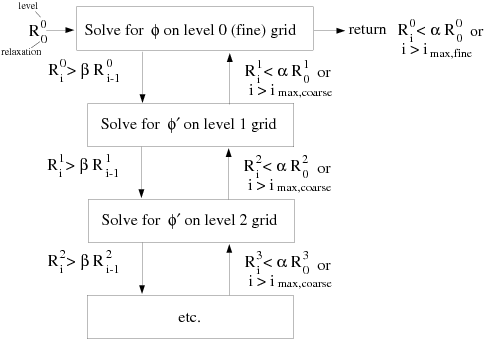
For the flexible cycle, the calculation and use of coarse grid
corrections is controlled in the multigrid procedure by the logic
illustrated in Figure 23.11: Logic Controlling the Flex Multigrid Cycle. This logic
ensures that coarser grid calculations are invoked when the rate of
residual reduction on the current grid level is too slow. In addition,
the multigrid controls dictate when the iterative solution of the
correction on the current coarse grid level is sufficiently converged
and should therefore be applied to the solution on the next finer
grid. These two decisions are controlled by the parameters  and
and  shown in Figure 23.11: Logic Controlling the Flex Multigrid Cycle, as described in detail below.
Note that the logic of the multigrid procedure is such that grid levels
may be visited repeatedly during a single global iteration on an equation.
For a set of 4 multigrid levels, referred to as 0, 1, 2, and 3, the
flex-cycle multigrid procedure for solving a given transport equation
might consist of visiting grid levels as 0-1-2-3-2-3-2-1-0-1-2-1-0,
for example.
shown in Figure 23.11: Logic Controlling the Flex Multigrid Cycle, as described in detail below.
Note that the logic of the multigrid procedure is such that grid levels
may be visited repeatedly during a single global iteration on an equation.
For a set of 4 multigrid levels, referred to as 0, 1, 2, and 3, the
flex-cycle multigrid procedure for solving a given transport equation
might consist of visiting grid levels as 0-1-2-3-2-3-2-1-0-1-2-1-0,
for example.
The main difference between the flexible cycle and the V and W cycles is that the satisfaction of the residual reduction tolerance and termination criterion determine when and how often each level is visited in the flexible cycle, whereas in the V and W cycles the traversal pattern is explicitly defined.
The multigrid procedure invokes calculations on the next coarser grid level when the error reduction rate on the current level is insufficient, as defined by
 | (23–131) |
Here  is the absolute sum of residuals
(defect) computed on the current grid level after the
is the absolute sum of residuals
(defect) computed on the current grid level after the  th relaxation on this level.
The above equation states that if the residual present in the iterative
solution after
th relaxation on this level.
The above equation states that if the residual present in the iterative
solution after  relaxations is greater than some fraction,
  (between 0 and 1), of
the residual present after the
(between 0 and 1), of
the residual present after the  th relaxation, the next
coarser grid level should be visited. Thus
th relaxation, the next
coarser grid level should be visited. Thus  is referred to as the residual
reduction tolerance, and determines when to "give up"
on the iterative solution at the current grid level and move to solving
the correction equations on the next coarser grid. The value of
is referred to as the residual
reduction tolerance, and determines when to "give up"
on the iterative solution at the current grid level and move to solving
the correction equations on the next coarser grid. The value of  controls the frequency
with which coarser grid levels are visited. The default value is 0.7.
A larger value will result in less frequent visits, and a smaller
value will result in more frequent visits.
controls the frequency
with which coarser grid levels are visited. The default value is 0.7.
A larger value will result in less frequent visits, and a smaller
value will result in more frequent visits.
Provided that the residual reduction rate is sufficiently rapid, the correction equations will be converged on the current grid level and the result applied to the solution field on the next finer grid level.
The correction equations on the current grid level are considered
sufficiently converged when the error in the correction solution is
reduced to some fraction,  (between 0 and 1), of the original error
on this grid level:
(between 0 and 1), of the original error
on this grid level:
 | (23–132) |
Here,  is the residual on the current
grid level after the
is the residual on the current
grid level after the  th iteration on this level, and
  is the residual that was initially obtained on this
grid level at the current global iteration. The parameter
is the residual that was initially obtained on this
grid level at the current global iteration. The parameter  , referred to as the
termination criterion, has a default value of 0.1. Note that the above
equation is also used to terminate calculations on the lowest (finest)
grid level during the multigrid procedure. Thus, relaxations are continued
on each grid level (including the finest grid level) until the criterion
of this equation is obeyed (or until a maximum number of relaxations
has been completed, in the case that the specified criterion is never
achieved).
, referred to as the
termination criterion, has a default value of 0.1. Note that the above
equation is also used to terminate calculations on the lowest (finest)
grid level during the multigrid procedure. Thus, relaxations are continued
on each grid level (including the finest grid level) until the criterion
of this equation is obeyed (or until a maximum number of relaxations
has been completed, in the case that the specified criterion is never
achieved).
The scalar AMG solver is used for the solution of linear systems obtained from the discretization of the individual transport equations.
 | (23–133) |
where the above equation contains scalar variables.
The coupled AMG solver is used to solve linear transport equations using implicit discretization from coupled systems such as flow variables for the density-based solver, pressure-velocity variables for the coupled pressure-based schemes and inter-phase coupled individual equations for Eulerian multiphase flows.
 | (23–134) |
where the influence of a cell  on a cell
  has the form
 | (23–135) |
and the unknown and source vectors have the form
 | (23–136) |
 | (23–137) |
The above resultant system of equations is solved in Ansys Fluent using either the Gauss-Seidel smoother or the Incomplete Lower Upper decomposition (ILU) smoother. If a scalar system of equations is to be solved then the point-method (Gauss-Seidel or ILU) smoother is used, while for a coupled system of equations the block-method (Gauss-Seidel or ILU) smoother is used.
The Gauss-Seidel method is a technique for solving a linear system of equations one at a time and in sequence. It uses the previously computed results as soon as they become available. It performs two sweeps on the unknowns in forward and backward directions. Both point or block method Gauss-Seidel smoothers are available in Ansys Fluent to solve for either the scalar AMG system of equations or the coupled AMG system of equations.
The Gauss-Seidel procedure can be illustrated using the scalar system, Equation 23–133. The forward sweep can be written as:
 | (23–138) |
where N is the number of unknowns. The forward sweep is followed by a backward sweep that can be written as:
 | (23–139) |
Following from Equation 23–138 and Equation 23–139, symmetric Gauss-Seidel can be expressed in matrix form as a two-step recursive solution of the system
 | (23–140) |
where  ,
,  , and
, and  represent
diagonal, lower tridiagonal, and upper tridiagonal parts of matrix
represent
diagonal, lower tridiagonal, and upper tridiagonal parts of matrix  , respectively.
Symmetric Gauss-Seidel has a somewhat limited rate of smoothing
of residuals between levels of AMG, unless the coarsening factor is
set to 2.
A more effective AMG smoother is based on the ILU decomposition technique. In general, any iterating method can be represented as
 | (23–141) |
where matrix M is some approximation of the original matrix A from
 | (23–142) |
 should be close to A and the calculation of
  should have a low operation count. We consider
  as an incomplete lower upper factorization of the matrix A such that
 | (23–143) |
where  and
and  are the lower tridiagonal and upper tridiagonal parts of matrix A. The
diagonal matrix D is calculated in a special way to satisfy the following condition for
diagonal
are the lower tridiagonal and upper tridiagonal parts of matrix A. The
diagonal matrix D is calculated in a special way to satisfy the following condition for
diagonal  of matrix M:
 | (23–144) |
In this case, the  th element of the diagonal of D will be calculated using
 | (23–145) |
The calculation of the new solution  is then performed in two symmetric recursive sweeps, similar to Gauss-Seidel
sweeps. Diagonal elements
is then performed in two symmetric recursive sweeps, similar to Gauss-Seidel
sweeps. Diagonal elements  of the ILU decomposition are calculated during the construction of levels
and stored in the memory. ILU smoother is slightly more expensive compared to Gauss-Seidel,
but has better smoothing properties, especially for block-coupled systems solved by coupled
AMG. In this case, coarsening of levels can be more aggressive using coarsening factors
between 8 and 12 for 3D problems compared to 2 for Gauss-Seidel.
of the ILU decomposition are calculated during the construction of levels
and stored in the memory. ILU smoother is slightly more expensive compared to Gauss-Seidel,
but has better smoothing properties, especially for block-coupled systems solved by coupled
AMG. In this case, coarsening of levels can be more aggressive using coarsening factors
between 8 and 12 for 3D problems compared to 2 for Gauss-Seidel.
Important: When solving the coupled systems, shorter solution times and more robust performance can be obtained by using the default ILU smoother, rather than the Gauss-Seidel smoother, which is the default for scalar systems. ILU is recommended whenever the coupled AMG solver is used. It is used by default for the coupled equations and, when a pseudo time method is selected, for the scalar equations.