5.2. Parts

5.2.1. Parts Quick Action Icons

Each of the several different types of parts share the following Quick Action Icons, which are used to adjust a number of attributes for individual parts.

Figure 5.6: Part Quick Action Icons

These are discussed here, but apply to all parts in Parts with a few exceptions. Those exceptions will be disclosed by the part attribute widget desensitized or invisible.

Part Visibility Icon

Determines the global (in all viewports and in all Modes) visibility of the selected Part(s).

Note: You can just right-click the part and choose Hide to make it invisible.

Figure 5.7: Part Visibility ON - OFF Icons

Part Color/Surface Property Icon

Clicking once on the Part Color/Surface Property icon opens a dialog which allows you to assign color, lighting characteristics, transparency levels, textures, and display surface flow to the individual Part(s) which has (have) been selected in the Parts list. If no Parts are selected, modifications will affect the default Part color and all Parts subsequently loaded or created will be assigned the new default color.

Note: You can just right-click a part and choose how to color it.

Figure 5.8: Part Color/Surface Property Icon

Figure 5.9: Part Color/Surface Property Dialog

Color By

Allows you to choose whether to color the selected Part(s) by a Constant Color or by a Variable.

Name
Column containing the name of the surface property (Constant or Variable name).
- Constant Color
  The selected Part(s) may be assigned a constant color by selecting it from the predefined matrix of color cells.
  - More...
    Alternatively, you can click on the More... area and the Select Color dialog will open.
    Figure 5.10: Select Color Dialog
    
    You can choose a color by entering RGB or HSV values directly, picking a color from the matrix, or custom color lists, or by utilizing the color square and slider. Regardless of which method you use to define a color, it will not be applied to the selected Part(s) until you click the OK button.
- Variable
  Alternatively, the Part(s) may be colored by a variable selected in the pulldown list. The color palette for each Variable associates a color with each value of the variable and these colors are used to color the selected Part(s).
  If coloring by a nodal variable, the default coloring will be continuously varying - even within a given element. If you are coloring by a per-element variable, the coloring will not vary within a given element. If you desire to see per-element variables in a continuously varying manner, you can toggle on Use continuous palette for per-element variables under Edit → Preferences... Color Palettes.
- Comp
  Column containing the component description for vector variables. The default component is Mag. If you are coloring by a vector variable clicking in its component column allows selection of the magnitude or its components (for example, X, Y, or Z).
  Figure 5.11: Part Color/Surface Property Editor Color by Vector Component
- Type
  The type of variable (blank is constant, scalar is single value at every node or element, vector is four values four values (three components and magnitude) at every node or element, tensor is six or 9 values at every node or element). Coordinates are a special client-side variable, with only magnitude available.

Edit Palette...

The Palette is the mathematical mapping of variable values to colors and to color opacity. Clicking on Edit Palette... will open the Palette Editor dialog and allow the editing of this mapping. See Edit Color Palettes.

Predefined Materials

Turn down exposes a number of predefined material models that allow you to quickly assign realistic surface model to part(s) without going through the trouble of adjusting the lighting and shading.

Note: After you pick a predefined material, you can still go to the lighting and shading turn down and further refine the settings. The lighting and shading options are context-sensitive to the predefined material you have selected.

Figure 5.12: Part Color/Surface Property Editor Predefined Materials

Default
Cloth
Glass
Metal
Paint
Plastic
Rubber

Lighting and Shading

Turn down exposes a number of detailed surface property controls that allow modification of detailed surface property attributes.

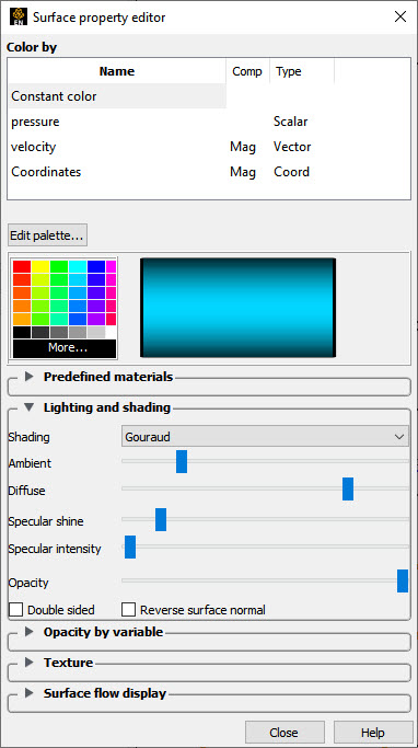
Figure 5.13: Part Color/Surface Property Editor Lighting and Shading

Shading
Selection of appearance of Part surface when Shaded Surface is on. Normally the mode is set to Gouraud, meaning that the color and shading will interpolate across the polygon in a linear scheme. You can also set the shading type to Flat, meaning that each polygon will get one color and shade, or Smooth which means that the surface normals will be averaged to the neighboring elements producing a smooth surface appearance. Not valid for all Part types. Options are:
- Flat
  Color and shading same for entire element.
- Gouraud
  Color and shading varies linearly across element.
- Smooth
  Normals averaged with neighboring elements to simulate smooth surfaces.
- Smooth High Quality
  Feature-based smoothing of adjacent elements within a fixed, internal threshold angle (30°).
Ambient
Controls the amount of natural surrounding light in an environment. A value toward 0.0 decreases (darkens) and toward 1.0 (floods) the amount of natural light.
Diffuse
The incoming light that will be reflected in all directions equally. The part will reflect no light if the value is 0.0, and will reflect maximum at 1.0 which diffuses the part surface color.
Specular Shine
Shininess factor. This is the dispersion angle of the reflected light. The larger the factor the smaller this angle. A large value of specular shine will therefore make the surface darker and appear less smooth because it more closely shows the changing normal along the surface.
Specular Intensity
Highlight intensity (the amount of white light contained in the color of the Part which is reflected back to the observer). Highlighting gives the Part a more realistic appearance and reveals the shine of the surface. To change, use the slider.
Opacity
This sets opacity as a constant percentage throughout the selected part(s). The opaqueness of the selected Part(s) applied as a constant value over the part surface. A value of 1.0 indicates that the Part is fully opaque, while a value of 0.0 indicates that it is fully transparent. Setting this attribute to a value other than 1.0 will adversely affect the graphics performance. Opacity is disabled for line parts.
Note: Opacity can be varied by constant, OR by a variable value in the Opacity By Variable turn down in this same dialog. This option will show up in the dialog only if you have opacity by variable set to constant (which is the default). In other words, you can use either this constant value of opacity OR you can set opacity by variable. You cannot do both. See Parts Quick Action Icons.
The term used in the graphics community for opacity is alpha. Alpha is a graphics term for the density or opaqueness of the color. Anytime the alpha is less than 1.0, the EnSight client calls into the graphics card’s rendering routines to perform complex calculations for rendering the translucent part. Note that setting a part’s opacity to transparent (0.0) will spend time and effort in the graphics card’s routines to render the chosen level of opacity, and is not the same thing as turning its visibility off using the visibility toggle (which simply does not render the part’s elements).
Double sided
Applies the lighting and shading properties to both sides of the surface element. Toggling OFF applies the lighting and shading properties only to the surface-normal side of the model elements.
Reverse surface normal
Reverses the surface normal on the surface element only on the client for lighting calculations when the Double sided toggled OFF. It does not modify the part for calculational purposes.

Opacity By Variable

This turndown allows you to control the opacity using a variable value, which can help to emphasize regions of importance, and de-emphasize uninteresting regions. This is an expensive calculation routine best run on a client machine with a good graphics card.

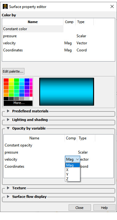
Figure 5.14: Part Color/Surface Property Editor Opacity by Variable

Note: You can't have opacity by a variable on a part while surface flow is being used on that part. As soon as you turn on surface flow, the Opacity by a variable alpha value will be reset to none.

Name
If this is set to constant opacity (which is the default), then the constant opacity under the Lighting and Shading dialog is enabled. In other words, you can use either this constant value of opacity or you can set opacity by variable. You cannot do both.
Choosing a variable name causes the opacity to vary according to the value of the variable and disables constant opacity under the Lighting and shading turndown.
If you wish to further increase or decrease the variable opacity by variable value, use the Palette Advanced tab as shown in the How to Set Surface Properties in Opacity by Variable (Transparency).
Comp
Column containing the component description for vector variables. The default component is Mag. If you are coloring by a vector variable clicking in its component column allows selection of the magnitude or its components (for example, X, Y, or Z).
Type
The type of variable (blank is constant, scalar is single value at every node or element, vector is four values at every node or element, tensor is six or 9 values at every node or element). Coordinates are a special client-side variable, with only magnitude available.

Texture

Texture mapping is a mechanism for placing an image on a surface or modulating the colors of a surface by various manipulations of the pixels via a texture map image. EnSight supports the application of a texture onto a part and the combining of texture effects with the normal EnSight coloring schemes. This can include animated textures (for example, .evo or .mpeg files), which can be used to texture parts and 2D annotations. Texture coordinates are computed via projection or using EnSight variables. Textures are loaded into EnSight, then they are applied to parts. This powerful capability is best explained using examples (see Map Textures).

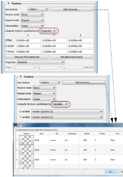
Figure 5.15: Part Color/Surface Property Editor Texture Main Dialogs

Use texture
Pick the texture number to use on the selected part. The texture number is set using the Edit textures... button just below.
Edit textures...
Click this button to open the Textures dialog. In the Textures dialog, right-click one of the numbered textures in the Texture column and choose an option as follows.
Figure 5.16: Part Color/Surface Property Editor Texture Editor
Right-click a texture
- Load texture...
  Load an image or a movie which can be used as a texture by choosing it in the Use texture pulldown above.
- Clear texture
  Clear the selected texture.
- Set border color...
  Each texture has a border color that is used for colors outside of the texture bounds. This color (RGB and opacity) can be set explicitly.
  Note: If Repeat mode is Repeat, then border color is not used. If Repeat mode is set to Clamp, then areas outside of the texture bounds will be clamped to the border color. If Repeat mode is set to Clamp to texture, then regions outside of the texture bounds will be clamped to the value just inside the texture.
- Set texture options...
  Open a dialog allowing you to set movie parameters: the start and end time, and the start and end frame, the compression methodology, and whether to autoscale time. This is useful to match up the movie end frames to the start and end of your timesteps which will synchronize your movie texture playback to your data timesteps.
- Display RGBA
  All textures have both a color (RGB) and an opacity (A) component. By default, the thumbnail is drawn using the full RGBA pixel value.
- Display RGB
  Display only the RGB portion of the thumbnail.
- Display Alpha
  Display only the alpha (opacity) of the thumbnail. Notice how the A channel masks out the black and white pixels in the RGB image. This masking can be used to place non-rectangular images/icons on EnSight parts.
Columns
- Dims
  Dimension of the texture/movie in pixels.
- File
  Path and filename to the texture image/movie.
- Transparent
  Yes/No indication of whether the texture uses transparency.
- Border
  Choose the border color around the texture used for colors outside of the texture bounds.
- Frames
  Number of frames in the texture (1 for image, >1 for movie).
- Time
  Static (image) or Transient (movie).

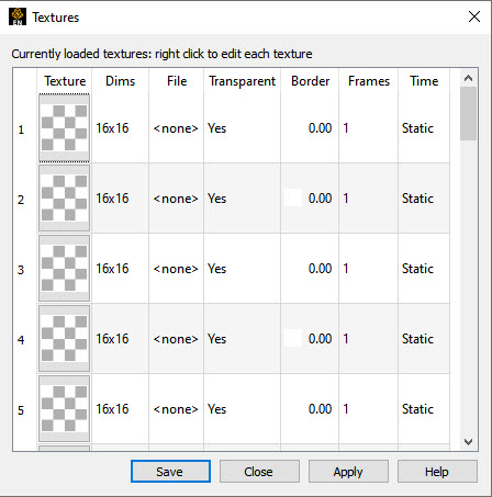
Save
Allows the user to save the currently loaded selection of textures and their display mode into your preferences directory. These will be automatically loaded every time EnSight is launched.

Texture mode
The texture mode determines how a texture is combined with the natural coloring scheme in EnSight. It has three values: Replace, Decal and Modulate.
- Replace
  In replace mode, the base colors provided by EnSight are ignored and the texture is used as the only source of color for the part
  Note: This has the side effect of disabling any lighting.
- Decal (default)
  In decal mode, the alpha channel of the texture is used to select between the texture color and the base color of the part. If the texture alpha value is 0, the base color of the part is displayed, while locations where the texture alpha value is 255, the texture color will be used exclusively. All alpha values in-between 0 and 255 will result in an interpolation between the texture and base colors.
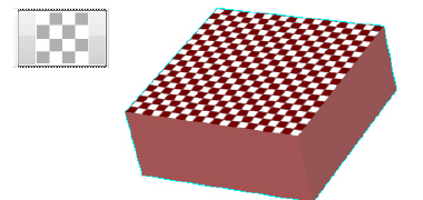
  Note: The default, checkerboard texture uses an alpha channel with values 255 and 80, which when applied to a reddish top surface will show up as follows. For details, see How to Place a Logo on a Part.
- Modulate
  In modulate mode, the base color is multiplied by the texture color and the resulting texture is used. Modulate mode is commonly used with a texture that has a color of white and some pattern in the alpha channel. This allows the base color to show through, but varies the transparency of the part. Arbitrary clipping operations can be set up this way. Modulation of the color channels can be confusing as the operation tends to suppress colors, but it can be used with a grayscale texture to attenuate. For details, see How to Clip an Object with a Texture.
Repeat mode
Repeat (default), Clamp, and Clamp to texture. When the current texture projection specifies texture coordinates outside of the texture [0,1], EnSight can either repeat the coordinates (for example, a texture coordinate of 2.3 is mapped to 0.3) or it can clamp to the border color of the texture. Clamping is often used for logos and explicit texture coordinates (See Texture Projections).
- Repeat
  Repeat the texture if outside the texture range [0,1]. If repeat mode is set to repeat, the border color of the texture is not used.
- Clamp
  Regions outside the texture range are fixed to the border color.
- Clamp to texture
  Regions outside the texture range are fixed to the texture just inside the border.
Interpolation
When the graphics hardware needs to access a pixel in the current texture it will either use interpolation or nearest neighbor.
- Nearest
  Nearest interpolation is more exact.
- Linear
  Bilinear interpolation is smoother and slower.
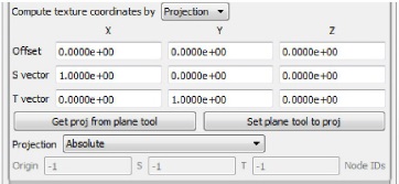
Compute texture coordinates by Projection
Projection (default), In projection mode, think of the texture as a projected light-source, like a presentation projector, only without divergence (i.e. the light lines are parallel). The user places the light source to shine through the scene at some orientation centered at some point. Textures are not limited to the exposed surface in EnSight, therefore any surface that intersects the beam of light is textured.
Figure 5.17: Part Color/Surface Property Editor Texture Coordinates by Projection
- Offset
  The Offset X,Y,Z values are considered to be relative to this node ID. If it moves in time, the texture projection will appear to be linked to it.
- S vector
  An offset for the S vector.
- T vector
  An offset for the T vector.
- Get proj from plane tool
  Get the projection using the plane tool orientation.
- Set plane tool to proj
  Set the plane tool position using the projection.
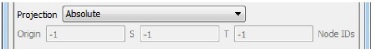
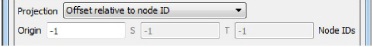
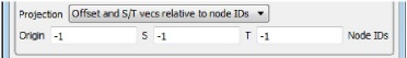
- Projection
  Three options: Absolute (default), Offset relative to node ID, and Offset and S/T vecs relative to node IDs.
  - Absolute (default) mode requires no input therefore the Origin, S, & T are grayed out. This will fix the texture to its absolute position and attitude in space. If the part geometry moves or deforms, the texture remains fixed in the scene, therefore it appears to slide along the part surface.
    Figure 5.18: Part Color/Surface Property Editor Texture Projection Absolute
  - Offset relative to node ID - The Offset relative to ID, allows you to specify a node ID in the Origin field so the texture will translate with the node id.
    Figure 5.19: Part Color/Surface Property Editor Texture Projection Relative Node ID
  - Offset and S/T vecs relative to node IDs - The Offset and S/T vecs relative to node IDs allows you to specify three node IDs that will be used to translate and rotate the texture in 3D space as these three nodes move: Origin, S & T.
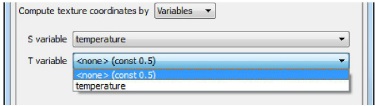
    Figure 5.20: Part Color/Surface Property Editor Texture Offset and S/T vecs Node IDs
Compute texture coordinates by Variables
In Variables mode, you must enter an S variable and a T variable and a pulldown for each of these variables will appear. In this mode, one or two scalar variables are used to provide explicit S and T texture coordinates for texturing. This is the most general mechanism for texturing. The S-variable and T-variable option menus provide a list of possible scalar variables. Users may also set the S and/or T value to the constant quantity 0.5. The variables are generally in the range [0,1], which map to the edges of the texture map, just inside the border. Values outside this range will either be mapped to the texture border color (in the case of clamp mode) or will be warped back into the range of [0,1] by repeated subtraction/addition (in repeat mode). This form of projection is capable of emulating the previous model. It also makes it relatively easy to create two dimensional data palettes. Just like the existing palette in EnSight, some function of a variable is used to select a color from a table. In this case, the table is a 2D texture, so this can be done for two different variables at the same time, and the opacity can be varied as a function of those variables.
Figure 5.21: Part Color/Surface Property Editor Texture Coordinates by Variables
- S variable
  Default is constant value (0.5). Select a variable with a range of [0,1],
- T variable
  Default is constant value (0.5). Select a variable with a range of [0,1],

Surface Flow Display

Toggles the display of Surface Flow Texture. This feature provides the capability to visualize a vector (typically velocity) over a surface part, similar to tufts in a wind tunnel. This is not the same as a particle trace part. It is a texture over the entire surface. The properties of a surface flow are per-case.

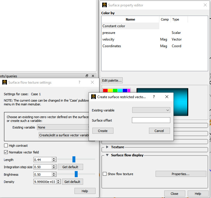
Figure 5.22: Part Color/Surface Property Editor Surface Flow Display

Show flow texture
This uses a Line Integral Convolution (LIC) algorithm to integrate a vector over a part surface. Select the part(s) on which you desire to display the surface flow, and toggle this ON (default OFF) to attempt to create a surface flow texture. If the chosen vector is zero at the surface then the surface flow texture will just be noise (and you may need to create a surface variable offset into the flow as described below). If the vector variable is per-element, the surface flow texture may not be smooth. You can use the calculator ElemToNode function to create a nodal variable and try again. Click the properties button to open the Surface Flow Texture Settings dialog which will give you more control of the result (see Surface Flow Display in How To Set Surface Properties ).
Properties
Click this button to open the Surface Flow Texture Settings dialog which will give you more control of the result.
- Existing variable
  Choose an existing vector variable to display on the surface as flow tufts.
- Create/Edit a surface vector variable
  If the vector variable is zero on the surface, then click this button to create a new variable from the flow field that can be displayed on the surface.
  Note: The first time you click this button, it will open the Create Surface Restricted Vector Variable dialog shown above. Choosing an existing variable and a Surface Offset will calculate a vector variable on the surface by mapping from the flow field using a pre-defined OffsetVar calculator function (See Variable Creation).
  The second time you click this button, it will open the calculator and allow you to edit the variable parameters themselves. You can just as easily calculate a variable using the OffsetVar function and use this variable in the Surface Flow display.
  Existing variable - pick an existing variable to offset into the flow.
  Surface Offset - pick a distance to offset into the flow, using the surface normal to get vector variable value.
- High Contrast
  Toggle this on to do a pass of image contrast enhancement. The resulting tuft lines will look sharper.
- Normalize Vector Field
  Toggle this on to normalize integration step length to the same unit length prior to visualization. This will result in all the tufts being the same length. With this off, the integration step length will be scaled according to the vector magnitude and areas where the vector magnitude is near-zero may contain algorithmic noise.
- Length
  The Line Integral Convolution (LIC) algorithm will integrate a maximum length of 20 pixel units in the positive and negative directions. Length is a scaling factor of this 20 pixels. Range is 0 to 1.
- Integration step size
  The step size in pixel units for each integration step. Range is 0 to 1.
- Brightness
  This will brighten up the surface flow tuft display.
- Density
  The density is a subjective value, related to the number of tufts on the surface. This value is inversely proportional to the model size, and is usually set to a very high initial value, which should create an acceptable flow pattern and may not need to be adjusted. The stepper will double and halve the step value. Above a certain value, there are diminishing returns from increasing this value.

Note: You can't have opacity by a variable on a part while surface flow is being used on that part. As soon as you turn on surface flow, the opacity by a variable alpha value will be reset to none.

LIC References:

Brian Cabral and Leith (Casey) Leedon. Imaging vector fields using line integral convolution. Proc of ISGGRAPH '93 (Anaheim, CA, Aug 1-6, 1993). In Computer Graphics 27, Annual Conference Series, 1993, ACM SIGGRAPH, pp 263-272.

Detlev Stalling and Hans-Christian Hege. Fast and resolution independent line-integral convolution. Proc of SIGGRAPH '95 (Los Angeles, CA, Aug 6-11, 1995). In Computer Graphics 29, Annual Conference Series, 1995, ACM SIGGRAPH, pp 249-256.

see https://en.wikipedia.org/wiki/Line_integral_convolution

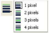
Part Line Width Icon

Opens a pulldown menu for the specification of the desired display width for Part lines. Performs the same function as the Line Representation Width field in the Node, Element, and Line Attributes section of the Feature Panel (Model).

Figure 5.23: Part Line Width Icon

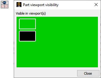
Part Visibility per Viewport Icon

Opens the Part Viewport Visibility dialog. If the global visibility of a Part is on, this dialog can be used to selectively turn on/off visibility of the selected Part(s) in different viewports simply by clicking on a viewport's border symbol within the dialog's small window. The selected Part(s) will be visible in the green viewports invisible in the black viewports.

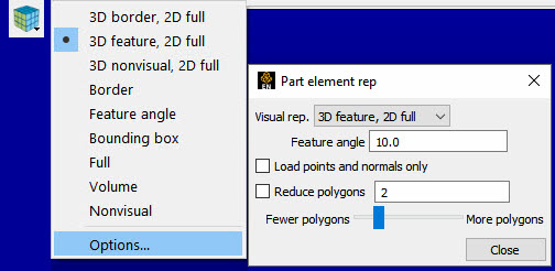
Figure 5.24: Part Visibility per Viewport Icon and Part Viewport Visibility Dialog

Part Element Settings Icon

Opens a pulldown for the specification of the desired representation for elements of the selected Part(s). Performs the same function as the Element Representation Visual Rep. pulldown menu in the Node, Element, and Line Attributes section of the Feature Panel (Model).

Figure 5.25: Part Element Settings Icon and Part Element Rep Dialog

Part Displacements Icon

Opens the Part Displacements dialog which allows you to choose the vector variable and displacement factor. The model geometry is displaced by this variable vector value.

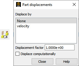
Displacement factor

The vector variable can be scaled by this factor.

Each node of a Part is displaced by a distance and direction corresponding to the value of a vector variable at the node. The new coordinate is equal to the old coordinate plus the vector times the specified Factor, or:

where C_new is the new coordinate location, C_orig is the coordinate location as defined in the data files, Factor is a scale factor, and Vector is the displacement vector.

Note: A value of 1.0 will give you true displacements.

You can greatly exaggerate the displacement vector by specifying a large Factor value. Though you can use any vector variable for displacements, it certainly makes the most sense to use a variable calculated for this purpose.

Note: The variable value represents the displacement from the original location, not the coordinates of the new location.

Displace Computationally

Displacements are done, by default, on the server (computationally). This means that the coordinates themselves are changed 'deeply' on the server and are used in calculations affected by the Coordinates (for example, Area, Volume, Length, etc). Toggling this off will make the displacements occur only on the client and not used for any computations.

Important: If you plan to use a computed variable for computational displacements, calculate the variable first, and then apply the computational displacements, so that all subsequent calculations will include the adjusted coordinates.

Modifying the coordinates from a variable computed from the coordinates will cause unexpected results as anytime the variable is computed it will be based on the adjusted coordinates of the part which will result in a displacement being applied multiple times. You can not use a displacement variable based on coordinates.

Visual Symmetry Icon

Opens the Part Visual Symmetry dialog which allows you to control the display of mirror images of the selected Part(s) or rotationally symmetric images about the Part's local frame axis and origin. This performs the same function as the Visual Symmetry menu in the General Attributes section of the Feature Panel (Model).

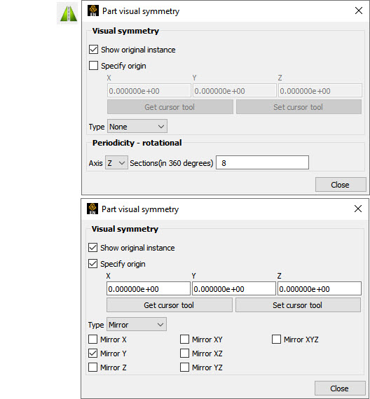
Figure 5.26: Visual Symmetry Icon and Dialogs

Symmetry enables you to reduce the size of your analysis problem while still visualizing the whole thing. Symmetry affects only the displayed image, not the data, so you cannot query the image or use the image as a parent Part. However, you can get the same effect by creating dependent Parts with the same symmetry attributes as the parent Part.

Show Original Instance

If toggled ON, the original instance will be visible. If toggled OFF, the original instance will not be visible.

Specify origin

You can specify the origin for the rotational or mirror symmetry.

Note: The default frame for all parts is frame 0 (which is coincident with the global axis). To quickly and easily modify the rotational origin, simply specify the origin in global coordinates. More complicated symmetries about axes not aligned with the global axes require assigning a new frame to the part(s) of interest.

Get/Set cursor tool

Populate the visual symmetry origin fields using the cursor tool location by clicking the get cursor tool button. Use the Set cursor tool button to assign the current origin field values to the cursor location.

Type

Mirror
3D space split by three planes of a cartesian frame (xy, xz, and yz) defines 8 quadrants
(+x+y+z, +x+y-z, +x-y+z, +x-y-z, -x+y+z, -x+y-z, -x-y+z, -x-y-z). Mirroring can be thought of as reflecting your model through these planes, or the origin, to get the proper mirrored image of the data in the various quadrants.
You can mirror the Part to more than one quadrant. If the Part occupies more than one quadrant, each portion of the Part mirrors independently. The images are displayed with the same attributes as the Part. For each toggle, the Part is displayed as follows. The default for all toggle buttons is OFF, except for the original representation - which is ON.
- Mirror X
  quadrant on the other side of the YZ plane.
- Mirror Y
  quadrant on the other side of the XZ plane.
- Mirror Z
  quadrant on the other side of the XY plane.
- Mirror XY
  diagonally opposite quadrant on the same side of the XY plane.
- Mirror XZ
  diagonally opposite quadrant on the same side of the XZ plane.
- Mirror YZ
  diagonally opposite quadrant on the same side of the YZ plane.
- Mirror XYZ
  quadrant diagonally opposite through the origin.
Rotational
Rotational visual symmetry allows for the display of a complete (or portion of a) "pie" from one "slice" or instance. You control this option with:
- Instances
  specifies the number of rotational instances to display.
  Note: An additional section appears for rotational symmetry only. It is entitled Periodicity - Rotational. While the Axis is used for both visual symmetry and periodic traces, the Sections field is only needed/used when periodic traces are created. See the Periodic Traces section of Create Particle Traces for instructions.
- Axis
  Specifies which rotational axis is to be used for rotational symmetry and periodic traces.
- Sections (in 360 degrees)
  Specifies the number of sections (instances) needed to make a full 360 degrees. Only used for periodic traces.
- Translational
  Translational visual symmetry allows for the display of a number of instance(s) of the model, each translated a fixed distance in the x, y, and/or z direction(s) from the previous instance.
- None
  No visual symmetry will be done.

Element Labeling Icon

Opens the Part Node/Elem Labelling dialog. Toggles on/off the visibility of the element and/or node labels (assuming the result file contains them) for the selected Part(s). The global Element Labeling Toggle (View → Label Visibility) must be on in order to see any element labels. Likewise, the global Node Labeling Toggle (View → Label Visibility) must be on in order to see any element labels.

Figure 5.27: Element Labeling Icon

Figure 5.28: Part Node/Elem Labeling Dialog

Figure 5.29: Filter Threshold Values

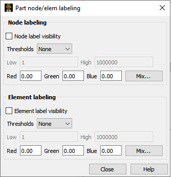
Element/Node Label Visibility

Toggles on/off the visibility of the element or node labels (assuming the result file contains them) for the selected Part(s). Performs the same function as the Label Visibility Node toggle in the Node, Element, and Line Attributes section of the Feature Panel (Model). Default is OFF.

Note: If your part geometry occludes your node ids then set the part opacity to transparent. To do this easily: Right-click the part in the graphics area, or on the selected part(s) in the part list and choose Color by → Make Transparent. To change it back, right-click and choose Color by → Make Opaque.

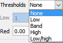
Filter Thresholds

A pulldown menu containing the following

Low
All element/node ids below the value in the low field are invisible
Band
All element/node ids between the values in the low and high fields are invisible.
High
All element/node ids above the value in the high field are invisible.
Low/High
All element/node ids below the low and above the high field values are invisible.

Red, Green, Blue, Mix

Enter the element/node id label color, or click the Mix button and pick your color.

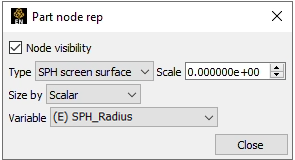
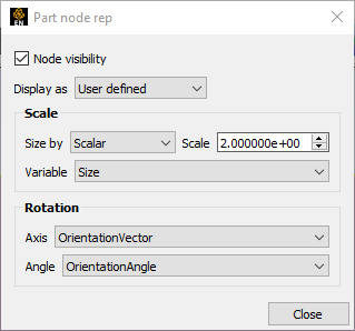
Node Representation Icon

Opens the Part Node Rep dialog. Performs the same function as the Node Representation area in the Node, Element, and Line Attributes section of the Feature Panel (Model).

Figure 5.30: Node Representation Icon

Figure 5.31: Part Node Rep Dialog

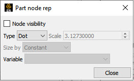
Node Visibility Toggle

Toggles-on/off display of Part's nodes whenever the Part is visible. Default is OFF.

Type

Opens a message menu for the selection of symbol to use when displaying the Part's nodes or point elements. Default is Dot. Options are:

Dot
To display nodes as one-pixel dots.
Cross
To display nodes as three-dimensional crosses whose size you specify. If you want to render as spheres, first choose Cross and get the Scale adjusted properly and then choose Sphere.
Sphere
To display the nodes as spheres. If your graphics card supports advanced GPU rendering of spheres (OpenGL version 3.3 or above) then the spheres will be rendered extremely efficiently and the detail box will be greyed out and unavailable.
Important: When rendered using advanced rendering, extremely large sphere sizes can cause greatly slow down rendering or even hang your graphics card (due to a driver limitation). Therefore, EnSight computes a safe sphere scale factor automatically as a starting point, and best practice is to use the up or down arrows to the right of the scale field to double or half the scaling value incrementally, then type in an exact value for fine adjustments.
SPH screen surface
Smoothed-particle hydrodynamics (SPH) is a meshless approach for simulating the mechanics of continuum media, such as solid mechanics and fluid flows. EnSight can display the SPH nodes as a surface efficiently rendered in the client’s screen space (more efficiently than on the server). Treating all the particles as a collection of spheres, the surface is extracted on the fly using a screen space voxel grid rendered into a surface. Therefore, real-time performance can be achieved. To use this feature, simply click the node representation icon and choose Type as SPH screen surface.
Note: For the best quality of surface reconstruction, you should set the size of particles correctly. It is best if you request that the solver exports the particle radius as a variable in the dataset; set the overall particle size to be twice the radius. If not, you can size by constant, starting with a small size and increasing it slowly, interactively until the visual result is satisfactory. Even with particle radius used, you may need to use a Scale smaller or larger than 2 to achieve the desired fluid-like surface. For more details on sizing the particle, see the following sections.
Since this approach internally uses the sphere rendering algorithm, the above limitations for sphere rendering also apply.
Figure 5.32: Sphere Rendering (Left), SPH Screen Surface Rendering (Right)

Scale
This field is used to specify the scaling factor for size of the node symbol. If Size By is Constant, this Scale field will specify the diameter of the marker in model coordinates. If Size By is set to a variable, this Scale field value will be multiplied by the variable value. If your variable is the particle diameter, then choose a Scale of 1.0 to see the appropriately scaled spherical representation of your particles, relative to the rest of the model. If your variable is the particle radius then choose a Scale of 2.0 to see the accurately scaled spherical representation of your particles relative to the rest of the model. Not applicable when the node-symbol Type is Dot.
Caution: Use caution here if using advanced GPU rendering of spheres because a large size relative to the size of the geometry can cause the graphics card to hang. Start out very small relative to the model size and use a cross instead of a sphere then increase your size until the crosses are sufficiently large, then change them over to spheres.
Size By
Opens a message menu for the selection of variable-type to use to size each node-symbol. For options other than Constant, the node-symbol size will vary depending on the value of the selected variable at the node. Not applicable when node-symbol Type is Dot. Get this working using Cross, then switch to Sphere to avoid hanging your graphics card. Default is Constant. Options are:
- Constant
  Sizes node using the Scale factor value.
- Scalar
  Sizes node using a scalar variable.
- Vector Mag
  Sizes node using magnitude of a vector variable.
- Vector X-Comp
  Sizes node using magnitude of X-component of a vector variable.
- Vector Y-Comp
  Sizes node using magnitude of Y-component of a vector variable.
- Vector Z-Comp
  Sizes node using magnitude of Z-component of a vector variable.
Variable
Selection of variable to use to size the nodes. Activated variables of the appropriate Size By type are listed. Not applicable when node-symbol Type is Dot or Size By is Constant.
User defined
For point parts, a reader can provide a mesh to be drawn for each node. When nodes are drawn this way, an orientation can also be applied. The orientation is defined by a vector variable and a scalar variable. The vector is an axis of rotation, and the scalar is an angle of rotation, in radians.
The reader for the Rocky solver is currently the only solver that provides a mesh per node and an orientation. All three attributes are applied automatically.

Filtered Elements Icon

Opens the Part Filter By Variable (Model parts only) dialog. Choose a variable (ideally a per-element variable, but you can also use a per-node variable which EnSight will average to the elements). This does a deep element removal of the elements from the selected model part on the server based on logical operators on the variable. Since filtering only works on model parts, filtering elements on a created part can only be accomplished by filtering them on the model parent part. Alternatively you can use the Filter part creation which will operate on a set of parent parts where those parent parts can be any part type.

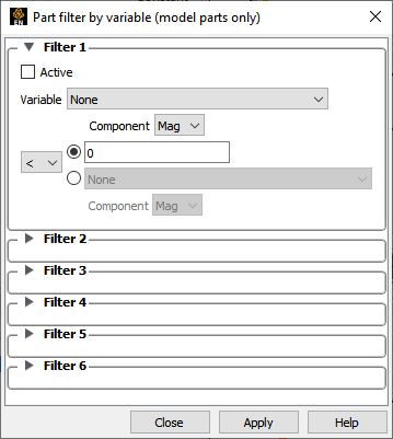
Six filters are available. Each filter can specify a variable to use in the filtering process which can be compared against another variable or a constant value. The filters are combined with and or or operators. The filtering occurs sequentially through the filters, that is, it is not possible, for example, to specify a filter operation of variable1 < 0.5 OR (variable2 > 1.0 AND variable 3 < 0.0)

See Filter Part Elements.

Variable

Select a scalar or vector variable.

Component

If a vector, then the component of the vector.

Active

Activate the filter by toggling it on. Notice that six filters can be toggled on.

And / Or

If you toggle on a logical operator then choose second threshold.

Part Element Blanking/Visibility Icon

Brings up the Part Element Blanking dialog. Element blanking is the visual removal of elements on the graphics screen. The elements still remain on the server and are still used in calculations, they are just not visible in the graphics window.

Note: Blanking is done using element IDs as tags. If the element IDs change each timestep, this can result in different elements becoming invisible each timestep.

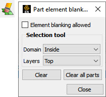
See Do Element Blanking.

Element blanking allowed

Toggles on/off whether element blanking allowed

Selection tool

Domain
Controls whether inside or outside of selection tool will be used fro the blanking
Layers
Controls the depth of the blanking operation. Top will just blank the first layer of elements encountered at each invocation. While all will blank elements at all depths.

Clear

Clears blanked elements and restores them to visible for the selected Part(s)

Clear all parts

Clears blanked elements and restores them to visible for all Part(s)

Part Shaded Surface Icon

Toggles on/off Shaded display of surfaces for the selected Part(s) assuming that global Shaded has been toggled ON in View → Shaded. Performs the same function as the Hidden Surface Toggle in the General Attributes section of the Feature Panel (Model). Default for all Parts is ON.

Figure 5.33: Part Shaded ON / OFF Icon

Part Hidden Line Icon

Toggles on/off hidden line display of surfaces for the selected Part(s) assuming that the global Hidden Line has been toggled ON in View → Hidden Line. Performs the same function as the Hidden Line Toggle in the General Attributes section of the Feature Panel (Model). Default for all Parts is ON.

Figure 5.34: Part Hidden Line ON / OFF Icon

Part Auxiliary Clipping Icon

Toggles on/off whether the selected Part(s) will be affected by the Auxiliary Clipping Plane feature. Performs the same function as the Aux Clip toggle in the General Attributes section of the Feature Panel (Model). Default is ON. Auxiliary clipping is simply a visual clipping that occurs only on the client and does not affect the underlying model geometry, only its view on the screen.

Note: The global Auxiliary Clipping Toggle (in View) must be on in order for any Parts to be affected by the Auxiliary Clip Plane.

Figure 5.35: Part Auxiliary Clipping ON / OFF Icon

Fast Display Representation Icon

Opens a pulldown menu for the specification of the desired fast display representation in which a Part is displayed. The Part fast display representation corresponds to whether the view Fast Display Mode (located in the View Menu) is on. The Fast Display pulldown icon performs the same function as the Fast Display pulldown menu in the General Attributes section of the Feature Panel (of all parts).

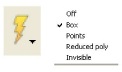
Figure 5.36: Fast Display Representation Icon

Box

Causes selected Part(s) to be represented by a bounding box of the Cartesian extent of all Part elements (default)

Points

Causes selected Part(s) to be represented by a point cloud

Reduced poly

Causes selected Part(s) to be represented by reduced number of polygons

Sparse Model

Decimates part elements by a factor determined in the Preferences. Go to Edit → Preferences → Performance and enter in a factor from 1 (sparse) to 100 (full) in the Sparse model representation field. This is only available when running in immediate mode using the -no_display_list option at startup.

Invisible

Causes the selected Part(s) to be invisible

(see General Attributes in Set Global Viewing Parameters).

5.2.2. Model Parts

When you start EnSight, you either read directly or interactively extract parts from the data files. Parts which come from the original dataset are referred to as model parts. Model parts are defined by the data readers and are usually a logical grouping of nodes and elements as defined by the solver. It might be a material or property or perhaps a defined geometric entity such as a wheel or inlet

The computational grid (or mesh) used by EnSight is either an unstructured definition (where each mesh element is defined) or a structured definition (an IJK definition) defining a rectilinear or curvilinear space. It is also possible to have a mixed definition where some parts are unstructured and other parts are structured.

When you read data you will choose the file name that will be read and set the format and options for the file. Then you will choose one of two options - either to load all the parts or to select parts to load.

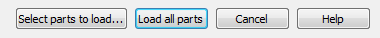
The Load all parts option will read the specified data (the case) and create (i.e. load) all of the parts into EnSight. The other option - Select parts to load... - will read the data but will not load any parts. This second option will allow you to select on a per part basis which parts will be loaded into EnSight. This load process is performed through the Part list.

The Part list contains all parts that have been read in (loaded) from your specified data file as well as those created within EnSight. Additionally, it may show model parts from the data that are not already loaded. These are referred to as Loadable Parts or LPARTS.

LPARTS may be loaded zero or more times. You may choose not to load a particular part from a data set if it is not needed for the visualization or analysis of the case. This is advantageous to save memory and processing time. You may also choose to load a part multiple times - so you could, for example, color the part by multiple variables at the same time in multiple viewports.

LPARTS are shown as grayed out parts in the Part list. You can load a LPART by selecting the part(s) and performing a right-click operation to Load part.

There are some creation attributes that affect model parts. These will be discussed in this section.

There are also various attributes that affect the display of these parts, as well as all created part types. These common attribute turndown sections of the Feature Panel, will also be described in this section.

Since Model Parts are controlled by the loading process, they have neither a specific Feature icon in the Feature Icon Bar, nor an entry in the Main Menu → Create menu. They do, however, have a Feature Panel associated with them. This Feature Panel for Model Parts is opened by double-clicking (or right-clicking and choosing Edit...) on a model part in the Part list.

Figure 5.37: Feature Panel - Model Parts

Figure 5.38: Advanced Feature Panel

Edit

Only the Edit mode is active, since all creation of model parts takes place with the loading process.

Note: When editing, the changes will be applied to those parts which have the small pencil icon next to them in the Parts list.

Advanced

Will open additional features for more advance control of the Part.

Desc

The name of the part being edited. You can modify this description as desired.

Creation

Creation Attributes for model parts consist of geometry scaling options (including server-side displacements) for unstructured and structured parts, and updating of I,J,K ranges for structured parts. Geometry scaling can be accomplished with a scale factor which will be applied to the model coordinates and/or a scale factor times a nodal variable. Updating the I,J,K node range attributes of the selected block structured Model Parts or the geometry scaling will cause proper updating of all dependent parts and variables.

Mesh
Opens pulldown menu for selection of model part re-meshing to use.
The default is to use the element connectivities described in the model data file(s). But a remeshing can be done, utilizing the QHull library. This library can compute the convex hull of point data, a 2D meshing. And since the convex hull of a 3D dataset lifted into 4 dimensional space turns out to be the volumetric tetrahedralization of the 3D data, it can be used to do a 3D meshing as well. Please note that this remeshing can take considerable memory and processing - so it needs to be used with that in mind. Also note, that if the model part has been used to create other, children parts, remeshing is not allowed. Only unstructured model parts are allowed to be remeshed. The following model parts are allowed: model, extract, point, and measured parts.
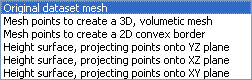
Also, the worst case for QHull is a large number of co-planar points. In the higher dimensional lifting step, the planarity adds a singularity that is difficult to work around. Using bounding boxes and planar projections can help. Accordingly, several options exist, which can be used if your data exhibits problematic characteristics. The pulldown menu options are:
- Original dataset mesh
  The nodes and elements described in the model data file(s) is used. No remeshing is done. This is the default.
- Mesh points to create a 3D, volumetric mesh
  The original element connectivities will be replaced with a volumetric meshing of the nodes of the part, to produce tet elements.
- Mesh points to create a 2D convex border
  The original element connectivities will be replaced with a convex hull meshing of the nodes of the part, to produce triangle elements.
- Height surface, projecting points onto YZ plane
  The original element connectivities will be replaced. The nodes of the part will be projected to the YZ plane and then triangulated in 2D. The resulting triangle element connectivities will be used with the original node data.
- Height surface, projecting points onto XZ plane
  The original element connectivities will be replaced. The nodes of the part will be projected to the XZ plane and then triangulated in 2D. The resulting triangle element connectivities will be used with the original node data.
- Height surface, projecting points onto XY plane
  The original element connectivities will be replaced. The nodes of the part will be projected to the XY plane and then triangulated in 2D. The resulting triangle element connectivities will be used with the original node data.
Note: There are a few formats that will not allow you to return to the input dataset elements once you have meshed the part. Most do. For these few (ABAQUS fil, Ansys, ESTET, Ansys FIDAP Neutral, Fluent Universal, and N3S), you can change between the 2D and 3D meshing options, but you need to delete the part and reload it, if you desire the part back to the input elements.

Improved Boundary Mesh

If one of the remeshing options is used, this toggle will employ a common trick that often helps with the co-planar points problem described above. The trick consists of adding 8 points (one at each corner of the bounding region) to the other points. This basically embeds the original points inside of an 8-point box. Then compute the volume tets and remove any tets connected to the non-original box points. Note that an offset can be used for the bounding region to ensure that the bounding region is not collapsed to 2D space (see Expansion factor below).

Expansion Factor
When adding the 8 points for the Improved boundary mesh trick above, an offset can be used to expand the bounding region in all directions. This is that offset, or expansion value.

Adjust Part Coordinates

The coordinates of the selected parts will be scaled and translated by the formula shown in the dialog. It is possible to apply a simple scale factor, and/or to apply a scaled nodal displacement vector variable (just choose the same vector variable for each pulldown and it will use the correct component). In fact each coordinate direction can be scaled according to a different model scalar variable if desired. This works only with model variables, not computed variables. This is server-side scaling and displacement, having the advantage of being able to properly query and compute on the displaced geometry of the model.

Other Options
If you want to displace by a vector in which the resulting displacement is updated each timestep then see Display Displacements.
If you want to scale the model coordinates visually only, then you can use the transform editor and choose the scaling option and visually scale the geometry in the three orthogonal directions, and do this separate for each direction (see Rotate, Zoom, Translate, Scale).
If you want to scale, translate, or rotate a number of parts visually only consider grouping them and doing a group transform (see Part Group Visual Transformations).
If you need to define your part(s) rotation or translation over time, consider rigid body translations (see EnSight Rigid Body File Format).
If you need precise control of the rotation and translation of parts separately for animation purposes, consider attaching a separate coordinate frame to each part (see Create and Manipulate Frames).

Change Structured Range and Step Values

The creation range and step values for structured parts can be changed here

IJK From
These fields specify the desired minimum interval value in the respective IJK component direction of the Model Part.
IJK To
These fields specify the desired maximum interval value in the respective IJK component direction of the Model Part.
IJK Step
These fields specify the desired interval stride value in the respective IJK component direction of the Model part.
IJK Min
These fields verify the minimum interval limit in the respective IJK component direction of the Model part.
IJK Max
These fields verify the maximum interval limit in the respective IJK component direction of the Model part.

(See Create IJK Clips).

Element Filters

Active
Enables Element Filtering.
Variable
Elements are removed from display on the client and from calculation on the server for model parts only, using the named variable (and component, if a vector) and the threshold operator(s) (< , > , = , != ) as well as the value (either a single number or another variable).
Note: Multiple filters can be applied sequentially strung together using logical ‘and’ or logical ‘or’:
Filtered elements are not removed when the geometry is saved in Case Gold format or as a Flatfile (see Saving Geometry and Results Within EnSight).

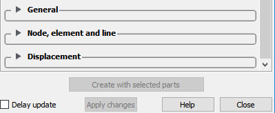
5.2.2.1. Feature Panel Turndowns Common To All Part Types

General

General attributes are general in that all Parts have them and they can't be neatly categorized into any other attribute type. Like all Part attributes, they are set individually for each Part.

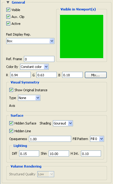
Visible
Toggles-on/off whether Part is visible on a global basis (in the Graphics Window or in all viewports). (Performs the same function as the Visibility Quick Action icon). Default is ON.
Aux. Clip
Toggles-on/off whether Part(s) selected in the Part list will be affected by the Auxiliary Clipping Plane feature, which enables you to make invisible that portion of each Part on the negative side of the current position of the Plane Tool. Performs the same function as the Auxiliary Clipping Quick Action icon. A Part with its Aux Clip attribute toggled-off will not be cut away. Default is ON. (See Set Auxiliary Clipping).
Active
Toggles-on/off whether or not display of the Part automatically updates as the solution time changes. When visualizing transient data, you may wish to freeze a Part in time while other Parts continue to update. For example, you can create two identical vector-arrow Parts, toggle-off Active for one of them, change the time step of the display and see how the vector arrows change from one time step to the other. Only the EnSight client Part is frozen, the EnSight server Part is kept current. Default is ON.
Visible in Viewport(s)
This small window allows you to control the visibility of the selected Part(s) on a per Viewport basis. Each visible viewport is shown. A green Viewport indicates that the selected Part(s) will be visible in this Viewport, while a black Viewport indicates that the selected Part(s) will not be visible. Change the visibility (black to green, green to black) by selecting a viewport with the mouse.
Fast Display Rep.
This pulldown menu allows for the selection of the fast display representation used to display a part on the client. This attribute helps the display of complex data sets. The part's fast display representation displays according to whether the global Fast display option (located in the View menu) is on or off and on the state of the Static Fast Display toggle located under Edit → Preferences..., Performance. For instance, when the Fast Display is Off (default) the part displays according to its specified Element Representation. When on, the parts are displayed by the fast display representation. The fast display representation will only be used while performing transformations, unless the Static Fast Display option has been selected. The part detail representations are:
- Off
  display according to specified Element Representation.
- Box
  a bounding (Cartesian extent) box of all part elements (default).
- Points
  point cloud representation of the part.
- Reduced poly
  polygon reduced representation of the part.
- Sparse Model
  display a percentage of the model in each display box (only available when running in immediate mode, using the -no_display_list startup option). You control this percentage in the performance preferences.
  Note: That it is useful for large models, but should probably not be used for small models.
- Invisible
  do not display at all while moving.
See Set Global Viewing Parameters.

Ref. Frame
This field specifies which frame the Part is assigned to. Default is the frame of the Part's parent Part (Frame 0 for original model Parts). Enter a different frame number in the field to change the assignment. Changing a Part's frame causes the Part to be drawn in the new coordinate frame. Once assigned to a different frame, the Part will transform with that frame. The choice of frame does not affect variable values. The interpolated value of a variable at point 0,0,0 in Frame 0 is the same as at point 0,0,0 in Frame 1, even though the points may appear at different locations in the Main View Window.
Color By
A pulldown menu for the selection of the variable color palette by which you wish to color the selected Part(s). Coloring a Part with a palette does not normally affect graphics performance while in line drawing mode, but Shaded Surface mode performance can be affected. If you do not color by a palette (Color By → Constant color), the Part will be displayed according to the color specified in the R, G, B fields. If you want to color Parts by palettes and want Shaded Surface mode, consider using the Static Lighting option (see Static Lighting in View Menu Functions).
RGB
These fields allow you to specify a solid color for the selected Part(s) (applicable only if Color By is Constant color). Enter a numerical value from 0 to 1 for each component color (Red, Green, and Blue).
Mix...
Opens the Select a color dialog for the selection of a solid color for the selected Part(s) (applicable only if Color By is Constant color).

Visual Symmetry

Allows you to control the display of mirror images of the selected Part(s) in each of the seven other quadrants of the Part's local frame or the rotationally symmetric instances of the selected parts. This performs the same function as the Visual Symmetry Quick Action icon.

Symmetry enables you to reduce the size of your analysis problem while still visualizing the whole thing. Symmetry affects only the displayed image, not the data, so you cannot query the image or use the image as a parent Part. However, you can create the same effect by creating dependent Parts with the same symmetry attributes as the parent Part.

Show Original Instance
Show the original instance or not
Type
- Mirror
  You can mirror the Part to more than one quadrant. If the Part occupies more than one quadrant, each portion of the Part mirrors independently. Symmetry works as if the local frame is Rectangular, even if it is cylindrical or spherical. The images are displayed with the same attributes as the Part. For each toggle, the Part is displayed as follows. The default for all toggle buttons is OFF, except for the original representation - which is ON.
  - Symmetry
    Mirror X - quadrant on the other side of the YZ plane.
    Mirror Y - quadrant on the other side of the XZ plane.
    Mirror Z - quadrant on the other side of the XY plane.
    Mirror XY - diagonally opposite quadrant on the same side of the XY plane.
    Mirror XZ - diagonally opposite quadrant on the same side of the XZ plane.
    Mirror YZ - diagonally opposite quadrant on the same side of the YZ plane.
    Mirror XYZ - quadrant diagonally opposite through the origin.
- Rotational
  Rotational visual symmetry allows for the display of a complete (or portion of a) pie from one slice or instance. You control this option with:
  Axis - rotates about the axis chosen.
  Angle - specifies the angle (in degrees) to rotate each instance from the previous.
  Instances - specifies the number of rotational instances.
- None
  No visual symmetry will be done.

Surface

Hidden Surface
Toggles on/off surface shading for individual Parts. When global Hidden Surface has been toggled on for the Graphics Window display (from View → Shaded or the global Shaded Surfaces Tools icon), individual Parts can be forced to stay in line drawing mode using this toggle. Default is ON. (see View Menu Functions).
Shading
Pulldown menu for selection of appearance of Part surface when Hidden Surface is on. Normally the mode is set to Gouraud, meaning that the color and shading will interpolate across the polygon in a linear scheme. You can also set the shading type to Flat, meaning that each polygon will get one color and shade, or Smooth which means that the surface normals will be averaged to the neighboring elements producing a smooth surface appearance. Not valid for all Part types. Options are:
- Flat
  Color and shading same for entire element
- Gouraud
  Color and shading varies linearly across element
- Smooth
  Normals averaged with neighboring elements to simulate smooth surfaces
- Smooth High Quality
  Uses the same algorithm as Smooth, except does not smooth sharp edges, which is useful if the user wants to retain some of the sharp features of the part.
Hidden Line
Toggles on/off hidden line representation for individual Parts. When global Hidden Line has been toggled on for the Graphics Window display (from View → Hidden Line or via the global Hidden Line Tools icon), individual Parts can be forced not to appear as Hidden Line representation using this toggle. (To have lines hidden behind surfaces, Parts must have surfaces, i.e. 2D elements) Default is ON. (see View Menu Functions)

Opaqueness
This field specifies the opaqueness of the selected Part(s). A value of 1.0 indicates that the Part is fully opaque, while a value of 0.0 indicates that it is fully transparent. Setting this attribute to a value other than 1.0 can seriously affect the graphics performance.

Lighting

Diff
This field specifies diffusion (minimum brightness or amount of light that a Part reflects). (Some applications refer to this as ambient light.) The Part will reflect no light if value is 0.0. If value is 1.0, no lighting effects will be imposed and the Part will reflect all light and be shown at full color intensity at every point. To change, enter a value from 0 to 1.
Shin
This field specifies shininess. You can think of the shininess factor in terms of how smooth the surface is. The larger the shininess factor, the smoother the object. A value of 0 corresponds to a dull finish and a value of 100 corresponds to a highly shiny finish. To change, enter a value from 0 to 100.
H Int.
This field specifies highlight intensity (the amount of white light contained in the color of the Part which is reflected back to the observer). Highlighting gives the Part a more realistic appearance and reveals the shine of the surface. To change, enter a value from 0 to 1 with larger values representing more white light. Will have no effect if Shin parameter is zero.
(see Set Attributes).

Volume Rendering

Structured Quality
This field controls the quality of volume rendering for a structured part. It allows a tradeoff between rendering speed and image quality. The Low, Medium, and High options provide this tradeoff by varying the number of samples. The Best option provides the most precise rendering by performing exact ray/cell intersections.
Node, element and line
Each Part's Node, Element, and Line attributes control the representation of the Part on the client, and how nodes, elements, and lines are displayed.

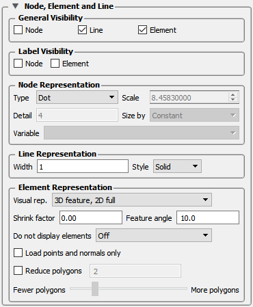
General Visibility
Node
Toggles-on/off display of Part's nodes whenever the Part is visible. Default is OFF.
Line
Toggles-on/off display of line (1D) elements in the client-representation whenever the Part is visible. Default is ON.
Element
Toggles-on/off display of 2D elements in the client-representation whenever the Part is visible.
Note: 3D elements are always represented as 2D elements on the client. Default is ON.
Label Visibility

Node
Toggles-on/off display of Part's node labels (if they exist) whenever the Part is visible. Only model Parts may have node labels. Default is OFF.
Element
Toggles-on/off display of Part's element labels (if they exist) whenever the Part is displayed in Full visual representation. Only model Parts may have element labels. Default is OFF.

Node Representation

Type
Opens a message menu for the selection of symbol to use when displaying the Part's nodes. Default is Dot. Options are:
- Dot
  to display nodes as one-pixel dots.
- Cross
  to display nodes as three-dimensional crosses whose size you specify.
- Sphere
  to display the nodes as spheres whose size and detail you specify.
- SPH Screen Surface
  Particles in an SPH point part are treated as spheres and a surface is extracted on the fly using a screen space voxel grid rendered into an outer surface.
Scale
This field is used to specify scaling factor for size of node symbol. Values between 0 and 1 reduce the size, factors greater than one enlarge the size. Not applicable when node-symbol Type is Dot. Default depends on your model size.
Detail
This field is used to specify how round to draw the spheres when the node-symbol type is Sphere. Ranges from 2 to 10, with 10 being the most detailed (for example,, roundest spheres). Higher values take longer to draw, slowing performance. Default is 2.
Size By
Opens a message menu for the selection of variable-type to use to size each node-symbol. For options other than Constant, the node-symbol size will vary depending on the value of the selected variable at the node. Not applicable when node-symbol Type is Dot. Default is Constant. Options are:
- Constant
  sizes node using the Scale factor value.
- Scalar
  sizes node using a scalar variable.
- Vector Mag
  sizes node using magnitude of a vector variable.
- Vector X-Comp
  sizes node using magnitude of X-component of a vector variable.
- Vector Y-Comp
  sizes node using magnitude of Y-component of a vector variable.
- Vector Z-Comp
  sizes node using magnitude of Z-component of a vector variable.
Variable
Selection of variable to use to size the nodes. Activated variables of the appropriate Size By type are listed. Not applicable when node-symbol Type is Dot or Size By is Constant.

Line Representation

Width
Specification of width (in pixels) of line elements and edges of 2D elements whenever they are visible. Range is from 1 to 20. Default is 1. Line widths other than 1 are not available on all hardware. This performs the same function as the Part Line Width Pulldown icon in Part Mode.
Style
Selection of style of line when lines are visible. Default is Solid. Options are:
Solid
Dotted
Dot-Dash

Element Representation

Visual Rep.
Selection of representation of Part's elements on the client. Saves memory and time to download.
- 3D border, 2D full
  represents the Part's 3D elements in Border representation, the Part's 1 and 2D elements in Full representation. The result is the outside surfaces of the Part are displayed along with all bar elements.
- 3D feature, 2D full
  represents the Part's 3D elements in Feature representation, the Part's 1 and 2D elements in Full representation. The result is the outside sharp edges of the Part are displayed along with all bar elements.
- 3D nonvisual, 2D full
  represents the Part's 3D elements in non visual representation, the Part's 1 and 2D elements in Full representation. The result is all the 1 and 2Delements from 2D parts are displayed.
- Border
  represents the Part's 3D elements with 2D elements corresponding to unshared element faces, the Part's 2D elements with 1D elements corresponding to the unshared edges, and the Part's 1D elements as 1D elements. The result is the outside faces and edges of the Part's elements.
- Feature Angle
  first runs the 3D border, 2D full representation to get a list of 1 and 2D elements. The 1D elements and all non-shared 2D edges will be shown, but only the shared edges above the Angle value will be shown. The result consists of 1D elements visualizing the sharp edges of the Part.
- Bounding Box
  represents all Part elements as a bounding box surrounding the Cartesian extent of the elements of the Part.
- Full
  represents all faces of the Part's 3D elements, and all the 1 and 2D elements.
- Non Visual
  means the Part exists on the server, but is not loaded on the client. Not Loaded Parts may be used as parent Parts, but do not exist on the client.
- Volume
  Represents a variable spatially by varying the alpha transparency according to the variable value throughout the spatial domain. This requires a modern graphics card.
Shrink Factor
Specification of scaling factor by which to shrink every element toward its centroid. Enter the fraction to shrink by in range from 0 to 1. Default is 0.0 for no shrinkage.
Angle
Specification of lower limit for not displaying shared edges in Feature Angle Representation. Value is in degrees.
Load points and normals only
Loads only vertex information and normals for the element representation given to the client. Useful for very large models.
Reduce Polygons
Lower the polygon density used to represent the part. Useful for very large models. Toggle on, then type in a value to reduce by, or slide the slider.
See Set Attributes and Display Labels

Displacement

Displacement Attributes specify how to displace the Part nodes based on a nodal vector variable. Each node of the Part is displaced by a distance and direction corresponding to the value of a nodal vector variable at the node. The new coordinate is equal to the old coordinate plus the vector times the specified Factor, or:

where:

C_new is the new coordinate location,

C_orig is the coordinate location as defined in the data files,

Factor is a scale factor, and

Vector is the displacement vector.

You can greatly exaggerate the displacement vector by specifying a large Factor value. Though you can use any vector variable for displacements, it certainly makes the most sense to use a variable calculated for this purpose.

Note: The variable value represents the displacement from the original location, not the coordinates of the new location.

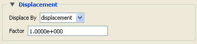
Displace By
Opens a message menu for selection of vector variable to use for displacement (or None for no displacement). Variable must be a nodal vector and be activated.
Factor
This field is used to specify a scale factor for the displacement vector. New coordinates are calculated as: C_new = C_orig + Factor*Vector, where C_new is the new coordinate location, C_orig is the original coordinate location as defined in the data file, Factor is a scale factor, and Vector is the displacement vector.
Note: A value of 1.0 will give you true displacements.
See Display Displacements.

IJK axis display

All Model and clip parts will have these attributes shown, but they only apply to those model and clip parts which are structured.

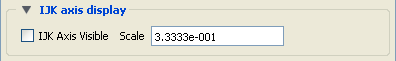
IJK Axis Visible
Toggle on to display an IJK axis triad for the part. IJK axis triad only visible when part is visible.
Scale
The scale factor for the IJK Axis triad.
(See Set Attributes).

5.2.3. Clip Parts

A Clip is a slice through one or more parts. This slice can be defined by a straight line; a plane; a quadric surface (cylinder, sphere, etc.); a constant x, y, or z value; a constant i, j, or k value; or a box. The clip can be created in selected model Parts or in previously created Clips, Isosurfaces, or Developed Surfaces. EnSight calculates the values of variables at the nodes of the Clip. Clips can also be parent Parts. For example, you can create a Clip Line passing through a vector field, then create vector arrows originating from the nodes of the Clip Line. Clips are created on the server, and so are not affected by the selected Representation(s) of the parent Part(s). If you activate or create variables after creating a Clip, the Clip automatically updates to include them.

You specify the location, orientation, and size of the Clip numerically in the Transformations Editor dialog, or interactively using the Line, Plane, Box, or Quadric surface tool. If you wish, EnSight will automatically extend the size of a Clip Plane to include all the elements of the parent Part(s) that intersect the plane.

A grid-clip ignores the mesh and creates a uniformly-spaced part with constant-sized elements. This allows you to sample variable values on a uniformly spaced grid. For a grid-type Clip Line, which is composed of bar elements, you specify how many evenly spaced nodes are along the line. For a grid-type Clip Plane, which is composed of rectangular elements, you specify the number of nodes in each dimension, resulting in an evenly spaced grid of nodes across the plane.

If you request a mesh-type Clip Line EnSight finds the intersection of the specified line with the selected parent Part(s) and creates bar elements that correspond to the mesh of the parent Part(s).

If you request a mesh-type Clip Plane, an xyz clip, or any of the quadric surfaces, EnSight finds the intersection of the specified plane or surface with the selected parent Part(s) and creates elements of various dimensions, sizes, and shapes that together form a cross-section of the parent Part(s). In this cross-section, three-dimensional parent Part elements result in two-dimensional Clip Plane elements, and two-dimensional parent Part elements result in one-dimensional Clip Plane elements.

Note: Two-dimensional parent Part elements that are coplanar with the cross-section are not included since they do not intersect the plane.

For line, XYZ, Plane, Quadric and Revolution Clips you can specify the resulting part to be all elements that intersect the specified value - resulting in a crinkly surface which can help analyze mesh quality.

For each Clip node on or inside an element of the selected parent Part(s), EnSight calculates the value of each variable by interpolating from the variable's values at the surrounding nodes of the parent Part(s).

You can interactively manipulate the location of a clip Part by toggling on the Interactive Tool button. When this toggle is on, the tool used to create the clip Part will appear in the Graphics Window. Manipulation of this tool will cause the clip Part to be recreated at the new location. This feature allows you to interactively sweep a plane across your model or manipulate the size and location of the cylinder, sphere, or cone.

You can animate a Clip by specifying an Animation Delta vector that moves the Clip to a new location for each frame or page of the animation. The Clip updates to appear as if it had been newly created at the new location and time.

For structured Parts, you can sweep through the Part with any of the i, j, or k planes.

A Box Clip will create a part according to the Box Tool. The result can either by the intersection of the Box Tool walls with the selected model parts (Domain = Intersect), the crinkly intersection of the Box Tool walls with the selected model parts (Domain = Crinkly), the portion of the selected parts that lie within (Domain = Inside) or outside (Domain = Outside) the Box Tool, a volume part (Domain = Volume), or a rectilinear clip of the selected parts that lie within the Box Tool.

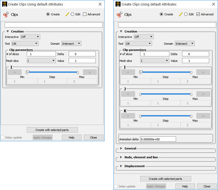
Clicking once on the Clip Feature icon (which be default is in the Feature Ribbon) or selecting Clips... in the Create menu, opens the Feature Panel for clip parts. This editor is used to both create and edit clip parts.

Figure 5.39: Clip Icon

Use Tool IJK

The IJK clip tool is used with structured mesh results.

Figure 5.40: Feature Panel - Clips - IJK

Create/Edit	Toggles that control whether a new part will be created, or whether you are editing existing part(s). Note: When editing, the changes will be applied to those parts which have the small pencil icon next to them in the Parts list.
Advanced	Will open additional features for more advance control of the Part.
Desc	The name of the part to be created or being edited.
Creation
Interactive	Opens pulldown menu for selection of type of interactive manipulation of the IJK clip. Options are:
	Off	Interactive IJK clips are turned off.
	Manual	Value of the IJK clip selected are manipulated via the slider bar and the IJK clip is interactively updated in the Graphics Window to the new value.
	Auto	Value of the IJK clip is incremented by the Auto Delta value from the minimum range value to the maximum value. When reaching the maximum it starts again from the minimum.
	Auto Cycle	Value of the IJK clip is incremented by the Auto Increment value from the minimum range value to the maximum value. When reaching the maximum it decrements back to the minimum.
Domain	Specification to extract the intersection of the specified mesh slice values. For IJK clips, the only valid selection is Intersect.
Clip Parameters
# slices	If you want more than one clip calculated at a Delta offset from each other, enter the number of slices in this field. This number of clips is calculated then they are grouped together. This field is only available at the first time the clip(s) are calculated. It is not possible to change this value and recalculate the clips. To change the number or the Delta, they must be deleted and recalculated.
Delta	Offset value to use for creating a number of clips. The first clip is calculated at the number entered in Value, and the next one is Delta + Value, etc. and they are all grouped together in the Part List.
Mesh Slice	Opens a pulldown menu for selecting which of the IJK dimensions you wish to allow to change. You will then specify Min, Max and Step limits for the two remaining fixed dimensions.
Value	This field specifies the I, J, or K plane desired for the dimension selected in Mesh Slice.
Slider Bar(s)	For IJK clips, the slider bar is used to increment / decrement the Mesh Slice Value between its Minimum and Maximum value.
	Min	Specification of the minimum slice value for the range used with the Manual slider bar and the Auto and Auto Cycle options.
	Max	Specification of the maximum slice value for the range used with the Manual slider and the Auto and Auto Cycle options.
	Step	Specification of the increment/decrement the slider will move within the min and max, each time the stepper buttons are clicked.
Animation Delta	This field specifies the incremental change in position of the clip for each page of Flipbook or frame of Keyframe animation.
Create with selected parts	Creates a Clip Part using the selected Part(s) in the Parts list.
Delay update	Checking this box will cause EnSight to not apply any changes made until you hit the Apply Changes button. When not checked, the changes are applied as you make them.

See Feature Panel Turndowns Common To All Part Types for a detailed discussion of the remaining Feature Panel turn-down sections which are the same for all Parts.

See Create IJK Clips.

Use Tool XYZ

The XYZ tool is used to create a planar Part at a constant Cartesian component value that is referenced according to the local frame of the part.

Figure 5.41: Feature Panel - Clips - XYZ

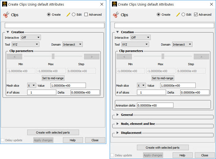
Create/Edit	Toggles that control whether a new part will be created, or whether you are editing existing part(s). Note: When editing, the changes will be applied to those parts which have the small pencil icon next to them in the Parts list.
Advanced	Will open additional features for more advance control of the Part.
Desc	The name of the part to be created or being edited.
Creation
Interactive	Opens pulldown menu for selection of type of interactive manipulation of the XYZ clip. Options are:
	Manual	Value of the XYZ clip selected are manipulated via the slider bar and the XYZ clip is interactively updated in the Graphics Window to the new value. For quick interactive control of the clip, simply left-click on the clip and grab the resulting green, cross-shaped click and go handle and drag left and right to see the clip value interactively decrease and increase respectively.
	Auto	Value of the XYZ clip is incremented by the Auto Delta value from the minimum range value to the maximum value. When reaching the maximum it starts again from the minimum.
	Auto Cycle	Value of the XYZ clip is incremented by the Auto Increment value from the minimum range value to the maximum value. When reaching the maximum it decrements back to the minimum.
Domain	Intersect	will create the cross section of the selected parts at the specified X, Y, or Z plane.
	Crinkly	will create a new part consisting of the parent part elements that intersect the X, Y, or Z plane.
Clip Parameters
Slider Bar	For XYZ clips, the slider bar is used to increment / decrement the Mesh Slice Value between its Minimum and Maximum value.
	Min	Specification of the minimum interval value of the interactive XYZ clip.
	Max	Specification of the maximum interval value of the interactive XYZ clip.
	Step	Specification of the interval step of the interactive XYZ clip.
Set to mid-range	Clicking this button will put the value that is halfway between the minimum and the maximum variable value.
Mesh Slice	Opens a pulldown menu for selecting which of the XYZ components you wish to clip, i.e. the X, the Y, or the Z component.
Value	This field specifies the coordinate desired for the Mesh Slice component.
# slices	If you want more than one clip calculated at a Delta offset from each other, enter the number of slices in this field. This number of clips is calculated then they are grouped together. This field is only available at the first time the clip(s) are calculated. It is not possible to change this value and recalculate the clips. To change the number or the Delta, they must be deleted and recalculated.
Delta	Offset value to use for creating a number of clips. The first clip is calculated at the number entered in Value, and the next one is Delta + Value, etc. and they are all grouped together in the Part List.
Animation Delta	This field specifies the incremental change in position of the clip for each page of Flipbook or frame of Keyframe animation.
Create with selected parts	Creates a Clip Part using the selected Part(s) in the Parts list.
Delay update	Checking this box will cause EnSight to not apply any changes made until you hit the Apply Changes button. When not checked, the changes are applied as you make them.

See Feature Panel Turndowns Common To All Part Types for a detailed discussion of the remaining Feature Panel turn-down sections which are the same for all Parts.

See Create XYZ Clips.

Use Tool RTZ

The RTZ tool is used to create a Part using cylindrical coordinates at a constant radius about an axis, angle around that axis or height along an axis.

Figure 5.42: Feature Panel - Clips - RTZ

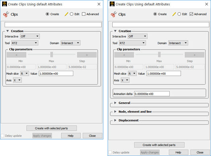
Create/Edit	Toggles that control whether a new part will be created, or whether you are editing existing part(s). Note: When editing, the changes will be applied to those parts which have the small pencil icon next to them in the Parts list.
Advanced	Will open additional features for more advance control of the Part.
Desc	The name of the part to be created or being edited.
Creation
Interactive	Opens pulldown menu for selection of type of interactive manipulation of the RTZ clip. Options are:
	Off	Interactive RTZ clips are turned off.
	Manual	Value of the RTZ clip selected are manipulated via the slider bar and the RTZ clip is interactively updated in the Graphics Window to the new value.
	Auto	Value of the RTZ clip is incremented by the Auto Delta value from the minimum range value to the maximum value. When reaching the maximum it starts again from the minimum.
	Auto Cycle	Value of the RTZ clip is incremented by the Auto Increment value from the minimum range value to the maximum value. When reaching the maximum it decrements back to the minimum.
Domain	Intersect	Will create a cross section of the selected parts at the specified radius, angle, or distance along the axis.
	Crinkly	Will create a new part consisting of the parent part elements that intersect the specified radius, angle or distance.
Clip Parameters
Slider Bar	For RTZ clips, the slider bar is used to increment / decrement the Slice Value between its Minimum and Maximum value.
	Min	Specification of the minimum slice value for the range used with the Manual slider bar and the Auto and Auto Cycle options.
	Max	Specification of the maximum slice value for the range used with the Manual slider and the Auto and Auto Cycle options.
	Step	Specification of the increment/decrement the slider will move within the min and max, each time the stepper buttons are clicked.
Mesh Slice	Opens a pulldown menu for selecting which of the RTZ components to clip, i.e. the radial (R), the angle theta (T) in degrees, or the distance along the longitudinal axis Z, (Z).
Value	This field specifies the magnitude desired for the Slice component, (theta in degrees).
Axis	The global axis with which to align the longitudinal (Z) RTZ axis.
Animation Delta	This field specifies the incremental change in position of the clip for each page of Flipbook or frame of Keyframe animation.
Create with selected parts	Creates a Clip Part using the selected Part(s) in the Parts list.
Delay update	Checking this box will cause EnSight to not apply any changes made until you hit the Apply Changes button. When not checked, the changes are applied as you make them.

See Feature Panel Turndowns Common To All Part Types for a detailed discussion of the remaining Feature Panel turn-down sections which are the same for all Parts.

See Create RTZ Clips.

Use Tool Line

The Line tool is used to create a clip line.

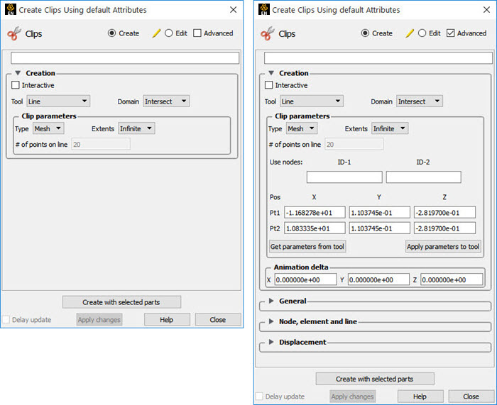
Figure 5.43: Feature Panel - Clips - Line

Create/Edit	Toggles that control whether a new part will be created, or whether you are editing existing part(s). Note: When editing, the changes will be applied to those parts which have the small pencil icon next to them in the Parts list.
Advanced	Will open additional features for more advance control of the Part.
Desc	The name of the part to be created or being edited.
Creation
Interactive	Toggles on/off interactive movement and updating of a clip Part. When toggled on, the line tool used to create the 2D clip line will appear in the Graphics Window. Movement of the tool will cause the Clip Part to be recreated at the new position. When manipulation of the tool stops, the clip Part and any Parts that are dependent on it will be updated. During movement, the Tool itself will not be visible, so as not to obscure the Line Clip Part. The Tool will reappear when the mouse button is released.
Domain	Specification to extract the intersection of the line tool with the selected part(s). For Line clips, the only valid selections are Intersect and Crinkly.
Clip Parameters
Type	Mesh	Will create a Line Clip showing the intersection of the line tool with the mesh elements of the parent Part.
	Extents	Opens a pull down menu for selection of the extent of the Line Clip. Finite limits the Line Clip to the length specified by the Line Tool endpoints. Infinite Assumes the line tool defines an infinite line and uses this to intersect the elements of the selected model Parts.
	Grid	Will create a Line Clip of evenly spaced bar elements along the line tool.
	# of Points on Line	Specification of number of evenly spaced points on the line at which to create a node.
Use nodes	Allows for specification of the location of two node ids in the model from which to get the line clip endpoints. If this method is used, the line clip will remain tied to these nodes even if they move over time.
Pos of Pt1, Pt2	Specification of XYZ endpoint-coordinates of Line Clip. The position of a Line Clip Part can be changed by manually entering values in the numeric fields and then pressing Enter.
Get Parameters from Tool	The values in the numeric fields (and the position of a Line Clip Part, if selected in the Feature Panel's Parts List) can be updated after moving the Line tool interactively in the Graphics Window by clicking Get Tool Coords. The Line Clip Part being edited will be repositioned to the new coordinates after clicking Get Tool Coords. Coordinates are always in the original model frame (Frame 0).
Apply Parameters to Tool	The position of the Line Clip tool can be changed by entering values in the numeric fields and then pressing Set Tool Coords.
Animation Delta
XYZ	These X,Y,Z fields specify the incremental change in position of the clip for each page of Flipbook or frame of Keyframe animation.
Create with selected parts	Creates a Clip Part using the selected Part(s) in the Parts list.
Delay update	Checking this box will cause EnSight to not apply any changes made until you hit the Apply Changes button. When not checked, the changes are applied as you make them.

See Feature Panel Turndowns Common To All Part Types for a detailed discussion of the remaining Feature Panel turn-down sections which are the same for all Parts.

(see Create Line Clips under Create Clips)

Use Tool Plane

Figure 5.44: Feature Panel - Clips - Plane

The Plane Tool is used to create a Plane Clip

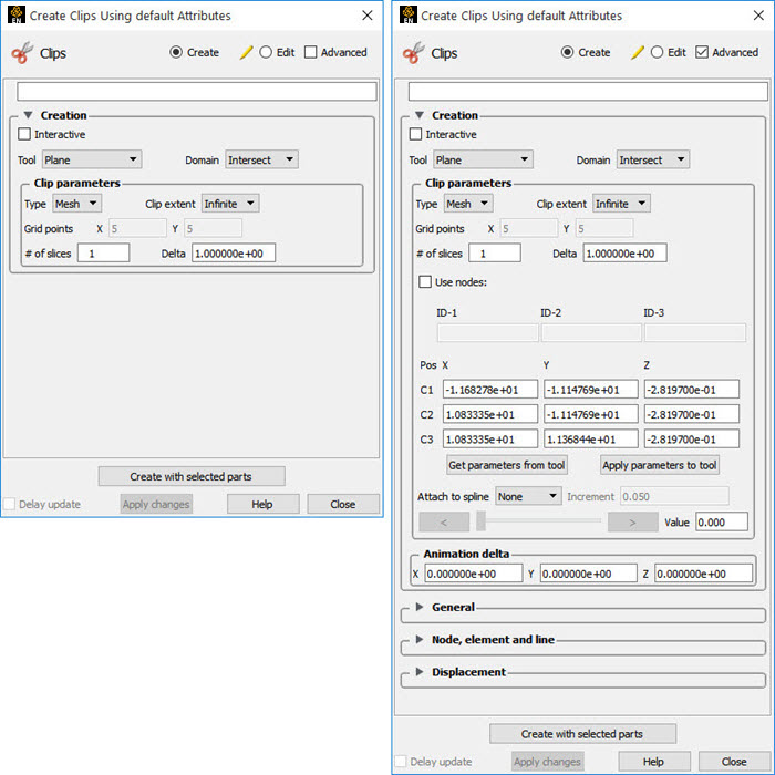
Create/Edit	Toggles that control whether a new part will be created, or whether you are editing existing part(s). Note: When editing, the changes will be applied to those parts which have the small pencil icon next to them in the Parts list.
Advanced	Will open additional features for more advance control of the Part.
Desc	The name of the part to be created or being edited.
Creation
Interactive	Toggles on/off interactive movement and updating of the clip Part. When toggled on, the Plane Tool used to create the clip Part will appear in the Graphics Window. Movement of the Plane Tool will cause the Plane Clip to be recreated at the new position. When manipulation of the tool stops, the clip Part and any Parts that are dependent on it will be updated. During movement, the Tool itself will not be visible, so as not to obscure the Line Clip Part. The Tool will reappear when the mouse button is released. For quick interactive control of the clip plane, simply left-click the plane tool origin and grab the resulting green, cross-shaped click and go handle and drag to see the clip location value interactively translate in the plane tool Z direction.
Domain	Intersect	will create the cross section of the selected parts where they intersect the plane tool.
	Crinkly	will create a new part consisting of the parent part elements that intersect the plane tool.
	Inside	will cut the parent parts and create a new part consisting of the portion on the positive z side of the plane tool.
	Outside	will cut the parent parts and create a new part consisting of the portion on the negative z side of the plane tool.
	In/Out	will cut the parent parts and create two new parts - namely an Inside and Outside part.
Clip Parameters
Type	Mesh	Will create a Plane Clip showing the cross section of the parent Part.
	Grid	Will create a Plane Clip of evenly spaced quad elements along the plane tool. These elements will be created via a remeshing of the parent parts.
	Grid Full	Will create a Plane Clip of evenly spaced quad elements along the plane tool. These elements are generated even if the parent parts does not have any element in the corresponding geometrical area, therefore creating a new domain if needed. The resulting clip will not contain any hole regardless of the geometry of the parent parts.
Clip extent	Finite	Limits the Plane Clip to the area specified by the Plane Tool corner coordinates.
	Infinite	Extends the Plane Clip to include the intersection of the plane with all elements of the selected model Parts.
Grid Pts on:XY	These fields specify the number of points on each edge of a Plane Clip at which to create nodes. Additional nodes are located in the interior of the plane to form an evenly spaced grid. The values must be positive integers. Applicable only to grid-type Plane Clips. Grid Pts in X correspond to the x-direction on the Plane tool, while the number of Grid Pts in Y correspond to the y-direction of the Plane tool.
# slices	If you want more than one clip calculated at a Delta offset from each other, enter the number of slices in this field. This number of clips is calculated then they are grouped together. This field is only available at the first time the clip(s) are calculated. It is not possible to change this value and recalculate the clips. To change the number or the Delta, they must be deleted and recalculated.
Delta	Offset value to use for creating a number of clips. The first clip is calculated at the number entered in Value, and the next one is Delta + Value, etc. and they are all grouped together in the Part List.
Use nodes	Specification of three node ids which will be used to specify the plane of the clip. The clip plane will be tied to these three nodes, even if they move in time.
Pos of C1,C2,C3	Specification of the location, orientation, and size of the Plane Clip using the coordinates (in the Parts reference frame) of three corner points, as follows: Corner 1 is corner located in negative-X negative-Y quadrant Corner 2 is corner located in positive-X negative-Y quadrant Corner 3 is corner located in positive-X positive-Y quadrant
Get Parameters from Tool	Will update the C1, C2, and C3 fields to reflect the current position of the Plane Tool.
Apply Parameters to Tool	Will reposition the Plane Tool to the position specified in C1, C2, and C3.
Animation Delta
XYZ	These X,Y,Z fields specify the incremental change in position of the clip for each page of Flipbook or frame of Keyframe animation.
Create with selected parts	Creates a Clip Part using the selected Part(s) in the Parts list.
Delay update	Checking this box will cause EnSight to not apply any changes made until you hit the Apply Changes button. When not checked, the changes are applied as you make them.

See Feature Panel Turndowns Common To All Part Types for a detailed discussion of the remaining Feature Panel turn-down sections which are the same for all Parts.

Create Clip Planes.

Use Tool Box

This Clipping Tool extracts portions of the model that are inside, outside, or that intersect a specified box.

Figure 5.45: Feature Panel - Clips - Box

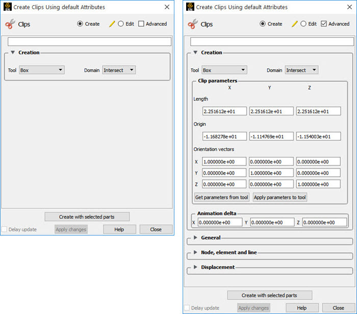
Be aware that due to the algorithm used, this clip can (and most often does) have chamfered edges, the size of which depends on the coarseness of the model elements

Create/Edit	Toggles that control whether a new part will be created, or whether you are editing existing part(s). Note: When editing, the changes will be applied to those parts which have the small pencil icon next to them in the Parts list.
Advanced	Will open additional features for more advance control of the Part.
Desc	The name of the part to be created or being edited.
Creation
Domain	Intersect	will create a new part consisting of the intersection of the box tool sides and the selected parts.
	Crinkly	will create a new part consisting of the parent part elements that intersect the box tool sides.
	Inside	will extract the volume portion of the parent parts that lie within the box.
	Outside	will extract the volume portion of the parent parts that do not lie within the box.
	In/Out	will create two new parts - namely the Inside and Outside parts.
	Volume	This option creates a client side volume rendering inside the box tool using the number of samples specified in the dialog in the x, y, and z directions. This allows volume rendering only in a specific portion of the selected part inside the box tool. In contrast, if you select the part and change its element representation to volume, then the entire geometry will be volume rendered. See the Element Representation section of Feature Panel Turndowns Common To All Part Types.
	Rectilinear	This option creates a server side rectilinear mesh using the box tool orientation and the number of samples specified in the dialog in the x, y, and z directions. Warning is given that this can be a performance and memory intensive part type.

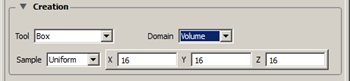	Sample	Type of sampling applied to the Box Tool: Uniform - Create a volumetric grid with the specified number of X, Y, and Z equally spaced divisions, or nodes along each axis - creating a uniform grid. X = The number of nodes along the x-axis of the box tool. Y = The number of nodes along the y-axis of the box tool. Z = The number of nodes along the z-axis of the box tool.
Clip Parameters
Length X,Y,Z	These fields specify the extent of the clip in the X, Y and Z dimensions.
Origin X,Y,Z	These fields specify the Origin of the clip in the X, Y and Z dimensions.
Orientation Vectors X,Y,Z	These fields contain the component values of the orthogonal box axis vectors.
Get Parameters from Tool	Will update the Origin and Orientation Vector fields to reflect the current position of the Box Tool.
Apply Parameters to Tool	Will reposition the Box Tool to the position specified in the Origin and Orientation Vector fields.
Animation Delta
XYZ	These X,Y,Z fields specify the incremental change in position of the clip for each page of Flipbook or frame of Keyframe animation.
Create with selected parts	Creates a Clip Part using the selected Part(s) in the Parts list.
Delay update	Checking this box will cause EnSight to not apply any changes made until you hit the Apply Changes button. When not checked, the changes are applied as you make them.

See Feature Panel Turndowns Common To All Part Types for a detailed discussion of the remaining Feature Panel turn-down sections which are the same for all Parts.

See Create Box Clips.

Use Tool Cylinder, Sphere, Cone

These Tools are used to create a quadric clip surface.

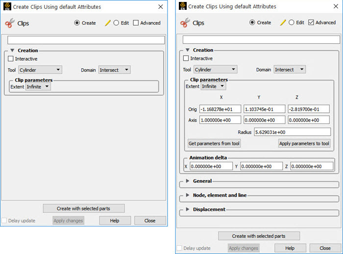
Figure 5.46: Feature Panel - Clips - Cylinder, Sphere, and Cone

Create/Edit	Toggles that control whether a new part will be created, or whether you are editing existing part(s). Note: When editing, the changes will be applied to those parts which have the small pencil icon next to them in the Parts list.
Advanced	Will open additional features for more advance control of the Part.
Desc	The name of the part to be created or being edited.
Creation
Interactive	Toggles on/off interactive movement and updating of a Clip Part. When toggled on, the Quadric Tool used to create the Clip Part will appear in the Graphics Window at the location of the Clip Part. Movement of the Quadric Tool will cause the Clip Part to be recreated at the new position. When manipulation of the tool stops, the Clip Part and any Parts that are dependent on it will be updated. During movement, the tool itself will not be visible, so as not to obscure the Line Clip Part. The tool will reappear when the mouse button is released.
Domain	Intersect	will create the cross section of the selected parts where they intersect the quadric tool.
	Crinkly	will create a new part consisting of the parent part elements that intersect the quadric tool.
	Inside	will cut the parent parts and create a new part consisting of the portion on the inside of the quadric tool.
	Outside	will cut the parent parts and create a new part consisting of the portion on the outside of the quadric tool.
	In/Out	will cut the parent parts and create two new parts - namely an Inside and Outside part.
	Note: If you clip through multiple parts, then you may not later change this domain.
Clip Parameters
Extent	Opens a pulldown menu that allows for the selection of Finite or Infinite extents. It is only present for cylinder and cone clips.
Clip Parameters
Cylinder	Orig	Specification of the origin (the center point) of the Cylindrical Clip.
	Axis	Specification of the longitudinal axis direction of the Cylindrical Clip.
	Radius	Specification of the radius of the Cylindrical Clip.
Sphere	Orig	Specification of the origin (the center point) of the Spherical Clip.
	Axis	Specification of the axis direction of the Spherical Clip. Note: Axis is important if Developed Surface is created from the spherical clip.
	Radius	Specification of the radius of the Spherical Clip.
Cone	Orig	Specification of the origin (the tip of the cone) of the Conical Clip.
	Axis	Specification of the axis direction of the Conical Clip. Axis direction goes from tip to base.
	Angle	Specification of the conical half angle (in degrees) of the Conical Clip.
Get Parameters from Tool	Will update the parameter fields to reflect the current position of the Tool.
Apply Parameters to Tool	Will reposition the Tool to the position specified in parameter fields.
Animation Delta
XYZ	These X,Y,Z fields specify the incremental change in position of the clip for each page of Flipbook or frame of Keyframe animation.
Create with selected parts	Creates a Clip Part using the selected Part(s) in the Parts list.
Delay update	Checking this box will cause EnSight to not apply any changes made until you hit the Apply Changes button. When not checked, the changes are applied as you make them.

See Feature Panel Turndowns Common To All Part Types for a detailed discussion of the remaining Feature Panel turn-down sections which are the same for all Parts.

See Create Quadric Clips.

Use Tool Revolution Tool

This Clipping Tool is used to create custom clip surfaces which are defined by revolving a set of lines about a defined axis.

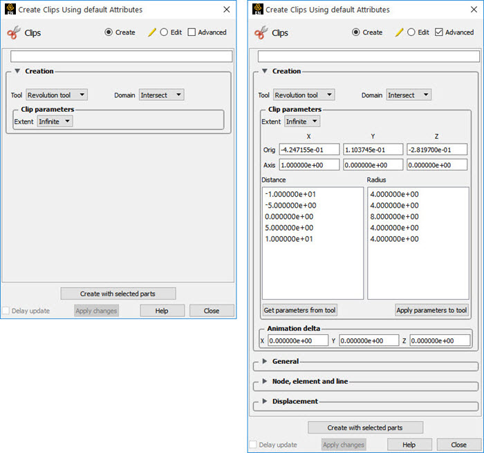
Figure 5.47: Feature Panel - Clips - Revolution

Create/Edit	Toggles that control whether a new part will be created, or whether you are editing existing part(s). Note: When editing, the changes will be applied to those parts which have the small pencil icon next to them in the Parts list.
Advanced	Will open additional features for more advance control of the Part.
Desc	The name of the part to be created or being edited.
Creation
Domain	Intersect	will create the cross section of the selected parts where they intersect the revolved surface.
	Crinkly	will create a new part consisting of the parent part elements that intersect the revolved surface.
	Inside	will cut the parent parts and create a new part consisting of the portion on the inside of the revolved surface.
	Outside	will cut the parent parts and create a new part consisting of the portion on the outside of the revolved surface.
	In/Out	will cut the parent parts and create two new parts - namely an Inside and Outside part.
	Note: If you clip through multiple parts, then you may not later change this domain.
Clip Parameters
Extent	Opens a pulldown menu that allows for the selection of Finite or Infinite extents.
Orig	Specifies the XYZ coordinates of the origin (center point) of the Revolution Clip.
Axis	These fields specify the XYZ coordinates of the axis direction of the Revolution Clip.
Distance/Radius	These lists specify the distance (from the origin) and radius for each point that defines the Revolution Clip. The points cannot be edited within this dialog. You must edit the Revolution Tool in the Transformations dialog.
Get Parameters from Tool	Will update the clip parameter fields to reflect the current position of the Revolution Tool.
Apply Parameters to Tool	Will reposition the Revolution Tool to the position specified in clip parameter fields.
Animation Delta
XYZ	These X,Y,Z fields specify the incremental change in position of the clip for each page of Flipbook or frame of Keyframe animation.
Create with selected parts	Creates a Clip Part using the selected Part(s) in the Parts list
Delay update	Checking this box will cause EnSight to not apply any changes made until you hit the Apply Changes button. When not checked, the changes are applied as you make them.

See Feature Panel Turndowns Common To All Part Types for a detailed discussion of the remaining Feature Panel turn-down sections which are the same for all Parts.

See Tools Menu Functions and Use Surface of Revolution Tool.

Use Tool Revolve 1D Part

This option will create a clip surface by revolving a line, defined by a Part, about an axis.

Figure 5.48: Feature Panel - Clips - Revolve 1D Part

Create/Edit	Toggles that control whether a new part will be created, or whether you are editing existing part(s). Note: When editing, the changes will be applied to those parts which have the small pencil icon next to them in the Parts list.
Advanced	Will open additional features for more advance control of the Part.
Desc	The name of the part to be created or being edited.
Creation
Domain	Intersect	will create the cross section of the selected parts where they intersect the revolved surface.
	Crinkly	will create a new part consisting of the parent part elements that intersect the revolved surface.
	Inside	will cut the parent parts and create a new part consisting of the portion on the inside of the revolved surface.
	Outside	will cut the parent parts and create a new part consisting of the portion on the outside of the revolved surface.
	In/Out	will cut the parent parts and create two new parts - namely an Inside and Outside part.
	Note: If you clip through multiple parts, then you may not later change this domain.
Clip Parameters
Revolve Part	This field specifies the Part number which will be revolved. The 1D Part must contain only bar elements and must have only two free ends (that is, there must be only one logical line contained in the Part).
Orig	These fields specify the XYZ coordinates of the axis line origin point.
Axis	These fields specify the direction vector of the axis line. The line contained in the Part specified by number in Revolve Part will be revolved about this axis to create the clip surface Part.
Animation Delta
XYZ	These X,Y,Z fields specify the incremental change in position of the clip for each page of Flipbook or frame of Keyframe animation.
Create with selected parts	Creates a Clip Part using the selected Part(s) in the Parts list.
Delay update	Checking this box will cause EnSight to not apply any changes made until you hit the Apply Changes button. When not checked, the changes are applied as you make them.

See Feature Panel Turndowns Common To All Part Types for a detailed discussion of the remaining Feature Panel turn-down sections which are the same for all Parts.

Use Tool General Quadric

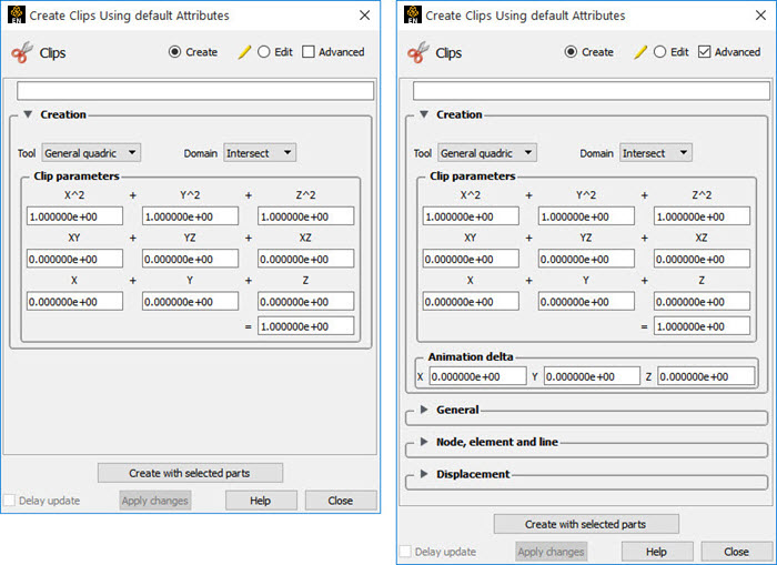
Figure 5.49: Feature Panel - Clips - General Quadric

Create/Edit	Toggles that control whether a new part will be created, or whether you are editing existing part(s). Note: When editing, the changes will be applied to those parts which have the small pencil icon next to them in the Parts list.
Advanced	Will open additional features for more advance control of the Part.
Desc	The name of the part to be created or being edited.
Creation
Domain	Intersect	will create the cross section of the selected parts where they intersect the general quadric surface.
	Crinkly	will create a new part consisting of the parent part elements that intersect the general quadric surface.
	Inside	will cut the parent parts and create a new part consisting of the portion on the inside of the general quadric surface.
	Outside	will cut the parent parts and create a new part consisting of the portion on the outside of the general quadric surface.
	In/Out	will cut the parent parts and create two new parts - namely an Inside and Outside part.
Clip Parameters
10 Coefficient Values	These coefficient values represent the general equation of a Quadric surface. They can be hanged by modifying the values. No tool exists corresponding to this equation.
Animation Delta
XYZ	Not available for General Quadric Clips.
Create with selected parts	Creates a Clip Part using the selected Part(s) in the Parts list.
Delay update	Checking this box will cause EnSight to not apply any changes made until you hit the Apply Changes button. When not checked, the changes are applied as you make them.

See Feature Panel Turndowns Common To All Part Types for a detailed discussion of the remaining Feature Panel turn-down sections which are the same for all Parts.

Use Tool Spline

This option will create a clip along an existing spline using evenly spaced nodes along the spline.

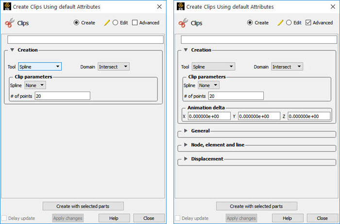
Figure 5.50: Feature Panel - Clips - Spline

Create/Edit	Toggles that control whether a new part will be created, or whether you are editing existing part(s). Note: When editing, the changes will be applied to those parts which have the small pencil icon next to them in the Parts list.
Advanced	Will open additional features for more advance control of the Part.
Desc	The name of the part to be created or being edited.
Creation
Domain	Intersect	will create the 1D part composed of bar elements using the selected parts where they intersect the spline at an evenly spaced number of points.
Clip Parameters
Spline	This pulldown allows you to choose which spline to use as the clipping tool.
# of points	Enter the number of evenly spaced points to use over the spline for the 1D clip creation.
Animation Delta
XYZ	These X,Y,Z fields specify the incremental change in position of the clip for each page of Flipbook or frame of Keyframe animation.
Create with selected parts	Creates a Clip Part using the selected Part(s) in the Parts list.
Delay update	Checking this box will cause EnSight to not apply any changes made until you hit the Apply Changes button. When not checked, the changes are applied as you make them.

See Feature Panel Turndowns Common To All Part Types for a detailed discussion of the remaining Feature Panel turn-down sections which are the same for all Parts.

Troubleshooting Clips

Problem	Probable Causes	Solutions
Clip does not move during animation	Animation deltas are not set, or are too small.	Change the animation delta values.
Clip results in an empty Part.	Clip was taken outside of the model.	Change the clip Tool location.

5.2.4. Contour Parts

Contours are lines that trace out constant values of a variable across the surface(s) of selected Part(s), just like contour lines on a topographical map.

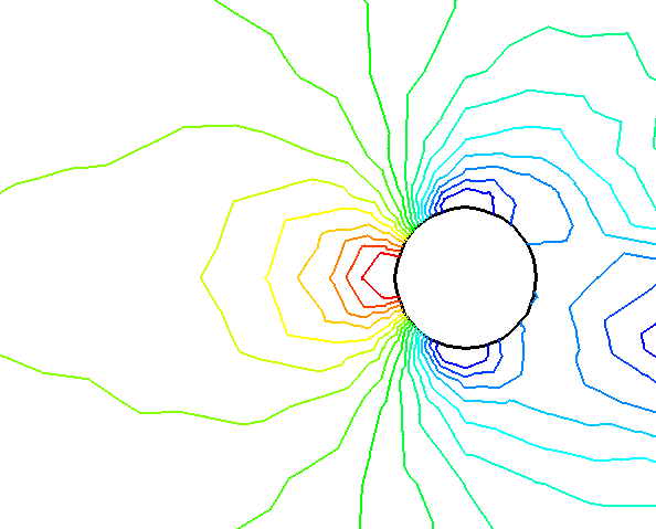
Figure 5.51: Pressure Contours in a Flow Field Around a Circular Obstruction

The variable must be a scalar or vector variable. If it is a vector, the magnitude or one of the components can be used. A Contour Part can consist of one contour line, or a set of lines corresponding to the value-levels of the variable palette. A Contour Part has its own attributes independent of those Parts used to create it (the parent Part(s)).

Contours are drawn across the faces of parent Part elements (one-dimensional elements are ignored). At each node along the edges of any one element face, the contour's variable has a value. If the range of these values includes the contour's value-level, the contour line crosses the face. EnSight draws the contour by dividing the face into triangles each having the face's centroid as one vertex. For each triangle the contour crosses, it will cross only two sides. EnSight interpolates to find the point on each of those two sides where the variable value equals the contour value-level, then creates a bar element to connect the two points.

Note: A contour line can bend while crossing an element face.

Because Contour Parts are created on the EnSight Client, the Representation attribute of the parent Part(s) greatly affects the result. Representations that reduce Part elements to one-dimensional representations (Border applied to two-dimensional Parts and Feature Angle), or do not download the Part (Not Loaded), will eliminate those Part elements from the Contour creation process. On the other hand, Full representation of three-dimensional elements will create contour lines across hidden surfaces. Usually, you will want the Representation selection to be 3D Border, 2D Full.

Contour Parts are created on the Client, and so cannot be queried or used in creating new variables. However, Contours can be used as parent Parts for Profiles and Vector Arrows.

If you have synced the contours to the variable palette and you change the value-levels in the Palette Editor, the Contour automatically regenerates using the new value-levels.

Use care when simultaneously displaying contours based on different function palettes so that you do not become confused as to which contours are which. Coloring them differently and adding an on-screen legend can help.

Left-clicking once on the Contours icon (or selecting Contours... from the Create menu) opens the Feature Panel for Contours in create mode. This editor is used to both create and edit contour Parts. Double-clicking on a part in the Parts list will open the Feature Panel for Contours in edit mode. Left-clicking the contour part in the graphics window will pop up a green handle. Drag this cross left and right to interactively change the contour density. Right-clicking on the contour part will give you a number of quick options, one of which is to right-click on a contour level and choose Label → Add to add a label at that location.

Figure 5.52: Contour Icon, and Create Menu Option

Figure 5.53: Feature Panel - Contours, Basic and Advanced

Create/Edit	Toggles that control whether a new part will be created, or whether you are editing existing part(s). Note: When editing, the changes will be applied to those parts which have the small pencil icon next to them in the Parts list.
Advanced	Will open additional features for more advance control of the Part.
Desc	The name of the part to be created or being edited.
Variable	Choose the variable to use for creating the contours from the pulldown.
Creation
Vector Component	If the variable chosen is a vector, choose magnitude or one of the X, Y, or Z components. Note: This is ignored if you use the advanced scaling option just described.
Sync To Palette	Toggles on/off the contour line synchronization to the legend color palette.
Color by creation	If toggled on at Contour part creation, then the Contour Part is colored by the variable.
Range Min	This field is activated when Sync to Palette Toggle is Off.
Range Max	This field is activated when Sync to Palette Toggle is Off.
Distribution	This pop-up menu is activated when Sync to Palette Toggle is Off. Opens a message menu for the selection of a distribution function for the contour lines. Choices include Linear, Logarithmic, and Quadratic.
Levels	This field is activated when Sync to Palette Toggle is Off. This field determines the number of contours between the Range Min and Range Max.
Visible	Toggles whether the main level contours are visible or not.
Sublevels	This field allows you to specify the number of sub-contours you wish to be drawn at evenly spaced value-levels between the value-levels defined above if not syncing to the palette, or defined in the Palette Editor if syncing to the palette. Leaving this field 0 will produce exactly the number of contour lines for which value levels are specified.
Visible	Toggles whether the sub-level contours are visible or not.
Display offset	Available in advanced mode, this field specifies the normal distance away from a surface to display the contours. A positive value moves the contours away from the surface in the direction of the surface normal. A negative value moves in the negative surface normal direction. Note: There is a hardware offset that will apply to contours, vector arrows, separation/attachment lines, and surface restricted particle traces that can be turned on or off in the View portion of Edit → Preferences. This preference (Use graphics hardware to offset line objects...) is on by default and generally gives good images for everything except move/draw printing. This hardware offset differs from the display offset in that it is in the direction perpendicular to the computer screen monitor (Z-buffer). Therefore, for viewing, you may generally leave the display offset at zero. But for printing, a non-zero value may become necessary so the contours print cleanly.
Labels	Available in advanced mode.
Auto Visible	Toggles on/off the visibility of the automatic number labels for contour lines.
Custom Visible	Toggles on/off the visibility of the custom number labels for contour lines. Custom labels are created at user-selected locations on the contour lines, using right-click at the desired contour location and choosing Labels → Add.
Delete all custom	Removes all custom number labels (which were created using right-click at a contour location and choosing Labels → Add).
Orientation	Determines the orientation between number labels: Tangential or Horizontal.
Font Size	Determines the number label font size.
Spacing	Determines the spacing between number labels.
Format	This pop-up menu allows selection of format of number labels. Choices include Exponential, and Floating Point.
Decimal Places	This field allows the specification of the number of decimal places of the number labels.
R,G,B	Allows the specification of red, green, and blue values for the assignment of a color to number labels.
Mix...	Opens the Color Selector dialog for the assignment of a color to number labels.
Create with selected parts	Creates a Contour Part using the selected Part(s) in the Parts list and the color palette associated with the variable currently selected in the Variables List.
Delay update	Checking this box will cause EnSight to not apply any changes made until you hit the Apply Changes button. When not checked, the changes are applied as you make them.
Apply Changes	Applies any changes made. Only active when Delay update is on.

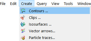
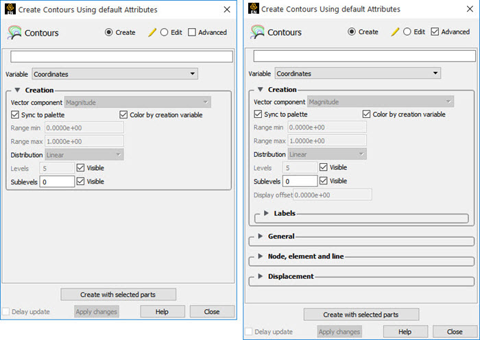
See Feature Panel Turndowns Common To All Part Types for a detailed discussion of the remaining Feature Panel turn-down sections which are the same for all Parts.

See Create Contours.

Troubleshooting Contours

Problem	Probable Causes	Solutions
No contours created.	Variable values on element faces are outside range of palette function value-levels.	Adjust palette function using the Palette editor if syncing to palette. Or adjust Range min and max in the Feature Panel if not syncing
No contours created.	Parent Parts do not contain any 2D elements.	Re-specify Parent Part list.
Too many contours.	Palette has too many function levels	Change the number of levels for the palette using the Palette editor if syncing to palette. Or adjust the levels in the Feature Panel if not syncing
Too many contours.	Specified too many sub-contours.	Lower the sub-contour attribute.
Too few contours.	The palette levels do not adequately cover the function value range for the Parent Parts.	Modify the palette using the Palette editor (if syncing) or the Feature Panel if not syncing.
Too few contours.	Sub-contour attribute set to 0.	Modify the Sub-contour attribute.
Contour Part created but (empty)	Parent Part is in Feature Angle representation.	Change Parent Part to 3D border, 2D full representation.
Contours are fine at first, but later go away.	Parent Parts representation changed to Feature Angle, or Not Loaded.	The contours are created from the Part representation on the EnSight client. Modifying the representation affects the Contour Parts.
Contour parts don't print well	See Display Offset above.	Enter a display offset (may need to be less than zero if viewed from backside).

5.2.5. Developed Surface Parts

A Developed Surface is generated by treating any 2D Part (or parent Part) as a surface of revolution, and mapping specific curvilinear coordinates of the revolved surface into a planar representation.

A Developed Surface derives its name from the implied process that defines a developable surface. A surface is considered developable if it can be unrolled onto a plane without distortion. Although every 2D Part in EnSight is not by definition a developable surface, each 2D Part can nevertheless be developed into a planar surface which is distorted according to the type of developed projection specified. For example, a Cylinder Clip Part is by definition a developable surface, because it can be developed into planar surface without distortion. Whereas, a Sphere Clip Part is not a developable surface, because it can not be developed into a planar surface without distortion.

5.2.5.1. Parent Parts

Only 2D Parts are developed. Also, only one Part is developed at a time. While all 2D Parts qualify as candidate parent Parts, only 2D Parts of revolution are developed coherently. The current developed surface algorithm treats all parent Parts as surfaces of revolution that are developed according to a local origin and axis of revolution. These attributes are either inherited from the parent Part, or must be specified according to the parent Part.

A developed surface permanently inherits the local origin and axis of revolution information from any parent Part created via the cylinder, cone, sphere, or revolution Clip tools. Whereas, surfaces developed from non-Clip Parts require this information to be specified via the Orig. and Axis fields in the Attributes (Developed Surfaces) dialog. The latter case is the only time the values in these fields are used. Although default values are provided, it is up to you to make sure that valid values are specified. In the former case, the Orig and Axis fields only provide convenient feedback of the selected Clip Part.

Note: Developed surfaces resulting from parent Parts of revolution created via the general quadric Clip tool do not inherit the local origin and axis of revolution attributes from the General Quadric Clip parent; rather, these attributes must be specified.

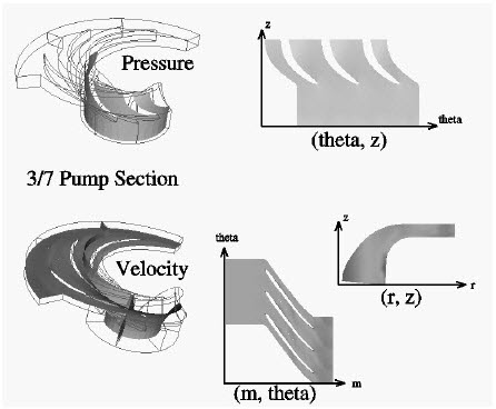
Figure 5.54: Developed Surface Examples

5.2.5.2. Developed Projections

A parent Part is developed by specifying one of five curvilinear mappings called developed projections; namely, an (r,z), (θ,z), (θ,r), (m,θ), or (m,r), projection. The curvilinear coordinates r, θ, z, and m stand for the respective radius, θ, z, and meridian (or longitude) directional components which are defined relative to the local origin and axis of revolution of the parent Part. The meridian component is defined as m = SQRT(r² + z²).

Essentially, each topological projection first surrounds the parent Part of revolution with a virtual cylinder of constant radius. The curvilinear coordinates of the parent Part are then projected along the normals of (and thus onto) the virtual cylinder. Finally, the virtual cylinder is slit along a straight line, or generator, and unwrapped into a plane. This process yields an equiareal, or area preserving, mapping which means that the area of any enclosed curve on the surface of the parent Part is equal to the area enclosed by the image of the enclosed curve on the developed plane. Although equiareal mappings provide reduced shape distortion, they do suffer from angular distortions of local scale.

Vector fields of the parent Part (for all three developed projections) are developed such that a vector’s angle to its surface normal is preserved. For example, a vector normal to the parent surface remains normal when developed onto the planar surface.

Figure 5.55: Developed Equiareal Projection

5.2.5.3. Seam Line

A surface of revolution is developed about its axis, starting at its seam line (or zero meridian) where the surface is to be slit. Surface points along the seam are duplicated on both ends of the developed Part. The seam line is specified via a vector that is perpendicular to and originates from the axis of revolution, and which points toward the seam which is located on the surface at a constant value. This vector can be specified either manually or interactively. Interactive seam line display and manipulation is provided via a slider in the Attributes (Developed Surfaces) dialog.

Clicking once on the Developed Surface icon (if you have customized the Feature Ribbon to have it visible) or selecting Developed Surfaces... in the Create menu, opens the Feature Panel for Developed Surfaces. This editor is used to both create and edit developed surface parts.

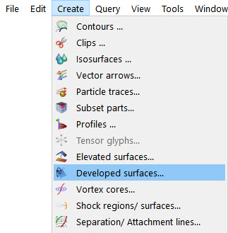
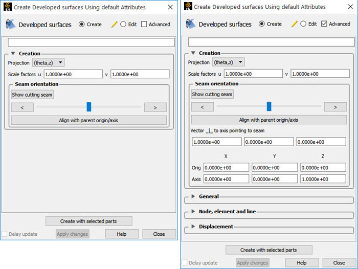
Figure 5.56: Developed Surface Icon, and Create Menu Option

Figure 5.57: Feature Panel - Developed Surfaces

Create/Edit	Toggles that control whether a new part will be created, or whether you are editing existing part(s). Note: When editing, the changes will be applied to those parts which have the small pencil icon next to them in the Parts list.
Advanced	Will open additional features for more advance control of the Part.
Desc	The name of the part to be created or being edited.
Creation
Projection	Opens a message dialog for the specification of which type of (u,v) projection, or mapping, you wish to use for developing a surface of revolution; where u,v denotes curvilinear components of the parent Part that are mapped into the xy-plane of reference Frame 0. The options are: (r,z) denotes the radial and z-directional components of the revolved surface. (theta,z) denotes the theta and z-directional components of the revolved surface. (theta,r) denotes the theta and radial components of the revolved surface. (m,theta) denotes the meridian and theta components of the revolved surface. The meridian component is the curvilinear component along a revolved surface that runs in the direction of its axis of revolution (for example, the meridonal and z-directional components along a right cylinder are coincident, and for a sphere the meridian is the longitude) (m,r) denotes the meridian and radial components of the revolved surface.
Scale Factors (u,v)	These fields specify the scaling factors which will be applied to the u and v projections.
Scale Factors (u,v)	These fields specify the scaling factors which will be applied to the u and v projections.
Seam Orientation
Show Cutting Seam	Click this button to display the current seam line location about the circumference of the revolved surface. The seam line is manipulated interactively via the Slider Bar.
Align with Parent Origin/Axis	Retrieves the Origin and Axis information from the Parent Part. Must be done if Parent Part is a quadric clip.
Vector _\|_ To Axis Pointing To Seam	These fields allow you to precisely specify the position of the Cutting Seam Line by specifying the direction of the vector perpendicular to the axis of revolution which points in the direction of the seam line.
Orig X Y Z	These fields specify a point on the axis of revolution.
Axis X Y Z	These fields specify a vector, which when used with the Axis Origin defines the axis of revolution.
Create with selected parts	Creates a Developed surface part using the selected Part(s) in the Parts list.
Delay update	Checking this box will cause EnSight to not apply any changes made until you hit the Apply Changes button. When not checked, the changes are applied as you make them.
Apply Changes	Applies any changes made. Only active when Delay update is on.

See Feature Panel Turndowns Common To All Part Types for a detailed discussion of the remaining Feature Panel turn-down sections which are the same for all Parts.

See Create Developed (Unrolled) Surfaces

Troubleshooting Developed Surfaces

Problem	Probable Causes	Solutions
Error message is encountered while creating a Developed Surface Part.	Parent Part is invalid.	Only 2D Parts can be developed.
Developed Surface is created, but is either not visible, Partially visible, or obstructed by other Parts which may be other developed Parts	Since all Developed Surfaces are projected about the origin on the xy-plane of the reference frame of the parent Part, they may map outside the viewport, intersect other Parts, or pile up on each other.	Set the Developed Surface to be viewed in its own viewport and initialize the viewport. Use different u/v scaling. Assign the developed Part to its own local reference frame and transform it accordingly.
Developed Surface Part is a line.	Wrong Projection type was specified.	Select a different Projection.
Developed Surface Part does not update to new Orig and/or Axis values.	The Orig and Axis values can not be specified if the Parent Part is created from either a cylinder, sphere, cone, or revolution quadric clip. These values can only be specified if the 2D parent Part is not a quadric clipped surface.	Since values entered for this condition are not used, click the Get Parent Part Defaults button to update the fields based on the selected parent Part in the Parts & Frames list.

5.2.6. Elevated Surface Parts

Elevated Surfaces visualize the value of a variable by creating a surface projected away from the 2D elements of the parent Part. An Elevated Surface might be used to show the pressure on a 2D surface representing the pressure as height above the 2D surface.

An Offset Surface projects an origin part into a 3D fluid domain using a single, fixed, translation vector and then interpolates a variable from the 3D domain onto the offset part. For example, an Offset Surface might be used to slightly offset the roof of a car in the vertical direction into the flow field to visualize the flow field velocity just outside of the boundary layer of the curved roof surface. Or, an Offset Surface might be used to translate an origin part into a 3D parent domain and clip the 3D domain using the origin part. Creation of an offset surface that results in a surface outside the 3D domain of the parent part(s) will result in significant performance delays as compared to a surface inside the 3D domain.

5.2.6.1. Elevated Surface

First let's look at the Elevated Surface. It is easiest to describe this feature if you think of a planar Part as the parent Part. Now warp this surface up out of plane proportionally to the value of a variable. The resultant surface is an Elevated Surface. Elevated surfaces are to surfaces what Profiles are to lines. While planar surfaces are perhaps the most useful parent Parts to use, parents do not have to be planar. Model Parts containing 2D elements, Clip Planes, Isosurfaces, and even other elevated surfaces are all valid parent Parts.

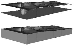
Figure 5.58: Elevated Surface Example, with and Without Sidewalls

The parent Part is not actually changed, a new surface is created. As this new surface is raised, projection (Sidewall) elements can be created stretching from the parent to the elevated surface around the boundary of the surfaces if desired. Just the surface, just the sidewalls, or both can be created.

The projection from a node on the parent Part will be in the direction of the normal at the node. If the node is shared by multiple elements, the average normal is used.

The projected distance from a parent Part's node to the corresponding elevated surface node is calculated by adding to the variable's value an Offset value, then multiplying the sum by a Scaling value. Adding the Offset enables you to shift the zero location of the plane. An Offset performs a shift, but does not change the shape of the resulting elevated surface. The Scaling factor changes the distance between parent and elevated surface, a "stretching" effect. EnSight will provide default values for both factors based on the variable's values at the parent Part's nodes.

5.2.6.2. Offset Surface

An offset surface requires two parts: an origin part and a 3D parent part. The origin part is offset by a single scaled vector into the 3D part and the offset part inherits the variable values of the 3D part at the intersection with the offset part. An example will help. Imagine you have the upper surface of an aircraft composed of 2D elements. The aircraft surface is enclosed within a 3D volume. The origin surface of the aircraft is shifted by the value of a user-supplied constant vector (and scale factor) into the 3D flowfield volume and becomes a new, Offset Part. The new Offset Part now inherits the 3D flowfield volume's variables at the new location of the surface. Offset functionality is effectively clipping a 3D volume using an origin part offset into the volume by a scaled, constant XYZ vector. You cannot scale, warp, or rotate the origin part. You can only translate it.

To use this function you must change the Elevated Surface default pulldown to Offset Surface. Then you must make sure you have selected the 3D volume parent part in the part list, and then enter the origin part in the field in the Feature Panel.

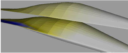
Figure 5.59: Offset Surface Example Above Main Model

Clicking once on the Elevated Surface icon (if you have customized the Feature Ribbon to have it visible) or selecting Elevated Surfaces... in the Create menu, opens the Feature Panel for Elevated Surfaces. This editor is used to both create and edit elevated surface parts.

Figure 5.60: Elevated Surface Icon

Figure 5.61: Feature Panel - Elevated Surfaces, Basic and Advanced

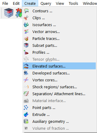
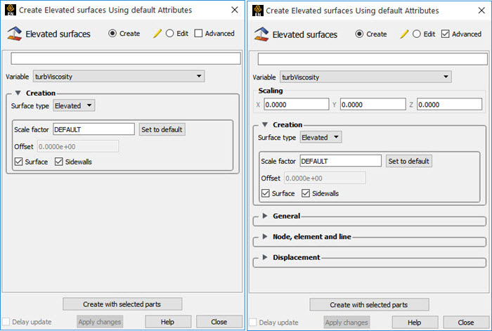
Create/Edit	Toggles that control whether a new part will be created, or whether you are editing existing part(s). Note: When editing, the changes will be applied to those parts which have the small pencil icon next to them in the Parts list.
Advanced	Will open additional features for more advance control of the Part.
Desc	The name of the part to be created or being edited.
Variable	Choose the variable to use for creating the elevated surface from the pulldown.
Scaling
XYZ	For vector-based or coordinate-based elevated surfaces, in advanced mode, specify vector components used in creating the elevated surface. Not applicable to scalar-type elevated surfaces. The scaling occurs according to the reference frame of the Elevated Surface-Part. Letters labeling dialog data entry fields depend on type of the reference frame (Rectangular, Spherical, or Cylindrical). If all components are 0.0, the vector or coordinate magnitude will be used. These are applied as:
Creation
Surface Type: Elevated	This pulldown chooses between Elevated Surface and Offset surface. Shown below are descriptions of the Elevated Surface options.
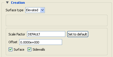Scale Factor	This field specifies the scaling for magnitude of distance between the parent Part node and the corresponding elevated surface node. The Factor is multiplied times the value of the variable. Values larger than one increase the size and values smaller than one decease the size. A negative value will have the effect of switching the direction of the projected surface
Set to Default	Click to set Scale Factor and Offset value to the calculated defaults based on the variable values for the parent Part.
Offset	Value specified is added to the variable values before the Scale Factor is applied to change the magnitude of projected distance. Default offset is magnitude of most-negative projection distance (will cause the surface to be projected positively). Has the effect of shifting the surface plot, but does not change the surface plot shape.
Surface Toggle	Toggles on/off the creation of the actual elevated surface. The sidewalls alone will be created if this toggle is off.
Sidewalls Toggle	Toggles on/off the creation of the sidewalls of the Elevated Surface. Elements will stretch from the parent Part to the Elevated surface around the boundary of the surfaces. The Elevated Surface alone will be created if this toggle is off.
Surface Type: Offset	This pulldown chooses between Elevated Surface and Offset surface. To use the Offset Surface option, you need to select the 3D volume part(s) in the main part window and set this pulldown surface type. Then set the options described below.
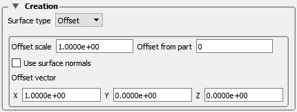Offset Scale	Scales the offset vector.
Offset Part	This field picks the origin part number that will be used to clip the volume part selected in the Part List.
Use Surface Normals	Use Surface normals of each element to create the offset surface.
Offset Vector	These fields are the rigid body translation vector for the entire offset origin part. The origin part cannot be scaled, warped, or rotated. Note: Letters labeling dialog data entry fields depend on type of the reference frame (Rectangular, Spherical, or Cylindrical).
Create with selected parts	Creates an elevated surface part using the selected Part(s) in the Parts list.
Delay update	Checking this box will cause EnSight to not apply any changes made until you hit the Apply Changes button. When not checked, the changes are applied as you make them.
Apply Changes	Applies any changes made. Only active when Delay update is on.

See Feature Panel Turndowns Common To All Part Types for a detailed discussion of the remaining Feature Panel turn-down sections which are the same for all Parts.

(See Create Elevated Surfaces).

Troubleshooting Elevated Surfaces

Problem	Probable Causes	Solutions
The entire Elevated Surface is not projected in the direction you want.		Change the sign of the scale factor.
You have a non-planar parent Part and the elevated surface seems to have strange intersecting elements.	Sidewall elements are not appropriate	Turn off sidewall toggle.
	Scale factor too large.	Lower the Scale Factor.
The Elevated Surface projection appears to be confused at various locations.	Inconsistently ordered elements, such that the normals are not consistent	Modify element ordering to be consistent, if possible.

5.2.7. Extruded Parts

Extruded parts are created by extruding a part in a directional or rotational manner to produce a part of next higher order. For example, a 2D axi-symmetric surface can be extruded rotationally about the proper axis to produce a 3D representation of the complete model. As another example, a 1D line can be extruded in a direction to produce a 2D plane.

Clicking once on the Extrude icon (if you have customized the Feature Ribbon to have it visible) or selecting Extrude... in the Create menu, opens the Feature Panel for Extruded parts. This editor is used to both create and edit extruded parts.

Figure 5.62: Extrusion Parts Icon

Figure 5.63: Feature Panel - Extruded Parts

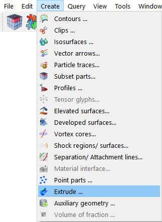
Create/Edit	Toggles that control whether a new part will be created, or whether you are editing existing part(s). Note: When editing, the changes will be applied to those parts which have the small pencil icon next to them in the Parts list.
Advanced	Will open additional features for more advance control of the Part.
Desc	The name of the part to be created or being edited.
Creation
Extrude by	Controls the type of extrusion to use.
	Rotation	To extrude the selected parts by revolving about an axis. This is what you would choose for an axi-symmetric part.
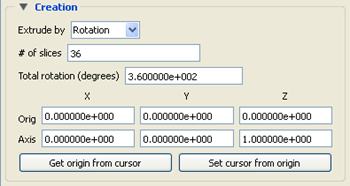	Translation	To extrude the selected parts by translating in a given direction.
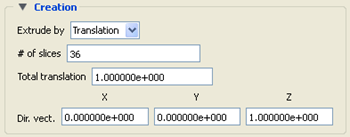# of slices	Sets the number of elements that will be created in the extrusion direction. For rotation, it would be the number of slices around the pie. For translation, it would be the number of elements along the extrusion vector direction.
Total rotation (degrees)	For rotation, sets the total number of degrees to rotate. It must be between -360 and +360.
Origin by Part Centroid	For rotation, sets x,y,z values for the origin of the axis of rotation using the part centroid to the part chosen in the Part ID field.
Origin	For rotation, sets x,y,z values for the origin of the axis of rotation.
Axis	For rotation, sets the direction vector components for the axis of rotation.
Cursor Get/Set	Can be used to get the origin values from the current cursor location, or to set the location of the cursor to be at the origin location.
Total translation	For translation, sets the total distance of extrusion travel.
Direction vector	For translation, sets the direction vector components for the directional extrusion.
Create with selected parts	Creates an extruded part using the selected Part(s) in the Parts list.
Delay update	Checking this box will cause EnSight to not apply any changes made until you hit the Apply Changes button. When not checked, the changes are applied as you make them.
Apply Changes	Applies any changes made. Only active when Delay update is on.

See Feature Panel Turndowns Common To All Part Types for a detailed discussion of the remaining Feature Panel turn-down sections which are the same for all Parts.

(see Parts Quick Action Icons and Extrude Parts).

Troubleshooting Extrusions

Problem	Probable Causes	Solutions
No extrusions created	Parent Part is not a valid server-side part.	Don't try to extrude client-side parts (particle traces, contours, etc.)

5.2.8. Isosurface Parts

Isosurfaces are surfaces that follow a constant value of a variable through three-dimensional elements. Hence, isosurfaces are to three-dimensional elements what contour lines are to two-dimensional elements.

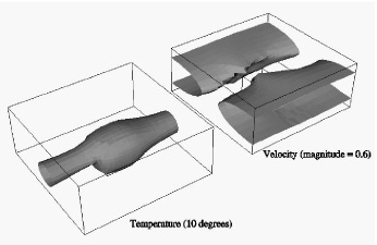
Figure 5.64: Isosurface Illustration

An isosurface may be based on a vector variable (magnitude or components), or a scalar variable. If the variable is elemental, then a temporary internal nodal variable is created by moving the elemental values to the nodes using simple averaging from the surrounding elements.

At each node of a three-dimensional element, the isosurface's variable has a value. If the range of these values includes the isosurface's isovalue, the isosurface cuts through the element. EnSight draws the isosurface through that element by first determining which edges the isosurface crosses, and then interpolating to find the point on each of those edges corresponding to the isovalue. EnSight connects these points with triangle elements passing through the parent Part elements. If the Parent Part(s) contain two-dimensional elements, a line is created across the elements - just like a contour.

All the triangle elements created inside all the three-dimensional elements of all the parent Part(s) together with all the lines created across the two-dimensional elements of all the Parent Part(s) constitute the isosurface. One-dimensional elements of the parent Part(s) are ignored. Because isosurfaces are generated by the server, the Representation of the parent Part(s) is not important.

You can interactively manipulate the value of an isosurface with a slider allowing you to scan through the min/max range of a variable. This scanning can also be done automatically. The isosurface will change shape as the value is changed.

If you are using animation, you can specify an Animation Delta value by which the isovalue is incremented for each animation frame or page. The isosurface is automatically updated to appear as if it had been newly created at the new location and time.

Left-clicking on the isosurface part in the graphics window will pop up a green handle in the shape of a cross. Drag this left and right to change the isosurface value. Right-clicking on the results in a pulldown menu of quick options for your isosurface.

Clicking once on the Isosurfaces icon (which be default is in the Feature Ribbon) or selecting Isosurfaces... in the Create menu, opens the Feature Panel for Isosurface parts. This editor is used to both create and edit isosurface parts.

Figure 5.65: Isosurfaces Icon

Figure 5.66: Feature Panel - Isosurfaces

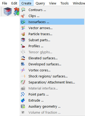
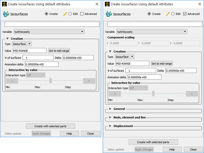
Create/Edit	Toggles that control whether a new part will be created, or whether you are editing existing part(s). Note: When editing, the changes will be applied to those parts which have the small pencil icon next to them in the Parts list.
Advanced	Will open additional features for more advance control of the Part.
Desc	The name of the part to be created or being edited.
Variable	Choose the variable to use for creating the isosurface from the pulldown.
Scaling
XYZ	For vector variables, in advanced mode, specify vector components used in creating the isosurfaces. Not applicable to scalar variables. Scaling occurs in the reference frame of the parent part. Letters labeling dialog data entry fields depend on type of the reference frame (Rectangular, Spherical, or Cylindrical). If all components are 0.0, the vector magnitude will be used. But, if any of these scaling factors is non-zero, the variable value will be computed as
Creation
Type
	Isosurface	Specification that an Isosurface type part created from the specified Variable and selected parts will have the isovalue of Value for all its elements.
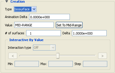	Isovolume	Specification that an Isovolume type part created from the specified Variable and selected parts will consist of elements with isovalues constrained to either below a Min, above a Max, or within the specified interval of Min and Max. The isosurface and isovolume algorithms are different. The isosurface algorithm defines the element intersection along the element surfaces. In contrast, the isovolume algorithm subdivides the 3D volume into tetrahedral elements and determines the intersections along the edges of each subdivided basis element resulting in more intersection points. For coarser meshes, the isosurface algorithm will be a smoother surface, but as the mesh gets finer the two algorithms should converge.
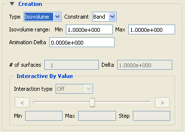Animation Delta	This field specifies the incremental change in isovalue for each frame or page of animation. It can be negative.
Value	Specification of numerical isovalue of the isosurface. To avoid an empty Part, this value must be in the range of the Variable within the Parent Parts. You can find this range using the Variables dialog or by showing the Legend for the Variable. For vector-variable-based isosurfaces, the vector magnitude is used.
Set to Mid-Range	Clicking this button will put the value that is halfway between the minimum and the maximum variable value.
# of surfaces	If you want more than one isosurface calculated at a Delta offset from each other, enter the number of surfaces in this field. This number of isosurfaces a1s calculated then grouped together. This field is only available the first time the isosurface(s) are calculated. It is not possible to change this value and recalculate the isosurfaces. To change the number or the Delta, they must be deleted and recalculated.
Delta	Offset value to use for creating a number of isosurfaces. The first isosurface is calculated at the number entered in Value, and the next one is Delta + Value, etc.
Constraint	Specification restricting the element isovalues of the Isovolume Part to an interval. The Constraint options are:
	Low	all elements of Isovolume Part have isovalues below the specified Min value.
	Band	all elements of Isovolume Part have isovalues within the specified Min and Max interval values.
	High	all elements of Isovolume Part have isovalues above the specified Max value.
Isovolume range Min	Specification of the minimum isovalue limit for the Isovolume Part
Isovolume range Max	Specification of the maximum isovalue limit for the Isovolume Part
Interactive By Value
Interactive Type	Opens pulldown menu for selection of type of interactive manipulation of the isosurface value. Options are: Off Interactive isosurfaces are turned off. Manual Value of the isosurface(s) selected are manipulated via the slider bar and the isosurface is interactively updated in the Graphics Window to the new value. For quick interactive control of the isosurface, simply left-click the isosurface and grab the resulting green, cross-shaped click and go handle and drag left and right to see the isosurface value interactively decrease and increase respectively. Auto Value of the isosurface is incremented by the Auto Delta value from the minimum range value to the maximum value. When reaching the maximum it starts again from the minimum. On some operating systems this may require the cursor to be in the Main View. Auto Cycle Value of the isosurface is incremented by the Auto Increment value from the minimum range value to the maximum value. When reaching the maximum it decrements back to the minimum.
Min	Specification of the minimum isosurface value for the range used with the Manual slider bar and the Auto and Auto Cycle options.
Max	Specification of the maximum isosurface value for the range used with the Manual slider and the Auto and Auto Cycle options.
Step	Specification of the increment/decrement the slider will move within the min and max, each time the stepper buttons are clicked.
Create with selected parts	Creates an isosurface part using the selected Part(s) in the Parts list.
Delay update	Checking this box will cause EnSight to not apply any changes made until you hit the Apply Changes button. When not checked, the changes are applied as you make them.
Apply Changes	Applies any changes made. Only active when Delay update is on.

See Feature Panel Turndowns Common To All Part Types for a detailed discussion of the remaining Feature Panel turn-down sections which are the same for all Parts.

Parts Quick Action Icons and Create Isosurfaces.

5.2.9. Material Interface Parts

EnSight enables you to create and modify Material Parts from material descriptions defined on model parts. The Material Parts feature allows you to extract single or combined regions of specified materials, as well as boundary interfaces between two or more specified materials.

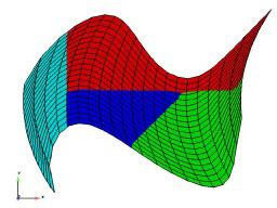
Figure 5.67: Material Parts Illustration

Material Parts can only be created from model parts that have material ids assigned to them. Therefore, Material Parts can not be created from any Measured or Created Parts. In addition, material information is not transferred to Created Parts.

Material Parts are created and reside on the server. They are Created Parts that provide proper updating of all dependent parts and variables - except they do not inherit any material data themselves.

Material Parts are created and modified by specifying parent model parts, as well as selecting material descriptions listed in the Materials List. A Material Part is extracted from only 2D and 3D elements. A Material Part is created as either a Domain or an Interface.

Domain

A material Domain defines a solid region composed of one or more specified materials. Parts with 2D elements yield 2D material elements, and parts with 3D elements yield 3D material elements.

Interface

A material Interface defines a boundary region between at least two or more adjacent specified materials. Parts with 2D elements yield 1D material elements, and parts with 3D elements yield 2D material elements.

Null Materials

Two categories of materials are reflected in the Materials List; namely, given materials and a null_material. All given material descriptions correspond to a material assigned a positive material number, or id. Any material that has an id less than or equal zero (<= 0) is grouped under the null_material and assigned the material id of zero (0). This allows the null material to act as a valid material. The null_material description always appears in the Materials List whether or not there are any null materials.

Formats

Materials may be defined either by the three sparse files (i.e. material ids, mixed ids, and mixed values), or materials may be designated as a set of per element scalar variable descriptions; but not by both. See EnSight Gold Casefile Format for format details.

Algorithm

Two algorithms are implemented to compute the material part: the smooth algorithm and the Young's algorithm. The smooth algorithm is based on a probability based approach to material interface reconstruction (see reference below). Essentially volume fractions are averaged for every cell to its nodes, edges/faces, and center. Each cell is then decomposed and/or subdivided into subcells. Each subcell is then repeatedly assigned, compared, and appropriately interpolated with volume fractions for each material. The resulting material cells reflect the maximum volume fraction portion(s) of the interpolated subcells.

The Young's algorithm partitions each mixed-material cell into regions which exactly match the material fractions. The partitioning is based on an orientation vector that determines the direction of the lines (or planes) used to subdivide the cell. Materials are sliced off in the order assigned by the user.

Reference

Meredith, Jeremy S. "A Probability Based Approach to Material Interface Reconstruction for Visualization", ECS277 Project 4, Spring 2001

D.L. Young, "Time-dependent multi-material flow with large fluid distortion," in Numerical Methods for Fluid Dynamics (K. W. Morton and J. J. Baines, eds.), pp. 273-285, Academic Press, 1982.

Caveats

Material resolution tends to diminish (and at times distorts) at boundary cells that lack adjacent ghost cells. The volume fractions at these cells simply lack the proper weighting. This is remedied by providing material ghost cells.

Therefore, materials that contribute half or less of the total portion on a boundary element, typically do not appear without ghost cells.

Specie(s)

Species may also be associated to a material (see MATERIAL under EnSight Gold Case File Format and EnSight Gold Material Files Format ), but are not involved in any of the computational aspects of creating/updating a material part. Rather, a material species variable may be created via the new variable calculator (see MatSpecies under Variable Creation).

Note: Species are only supported with the three sparse material files format, and are not supported by the materials as scalars per element format.

Access

Clicking once on the Material Interface icon (if you have customized the Feature Ribbon to have it visible) or selecting Material Interface... in the Create menu, opens the Feature Panel for Material parts. This editor is used to both create and edit Material interface parts.

Figure 5.68: Material Parts Icon

Figure 5.69: Feature Panel - Material Parts

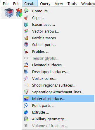
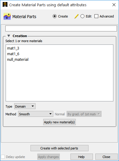
Create/Edit	Toggles that control whether a new part will be created, or whether you are editing existing part(s). Note: When editing, the changes will be applied to those parts which have the small pencil icon next to them in the Parts list.
Advanced	Will open additional features for more advance control of the Part.
Desc	The name of the part to be created or being edited.
Creation
Materials List	List reflecting the available materials in the model parts. Any material that has an id less than or equal to zero (<= 0) comprises the null_material.
Type	Opens a pulldown menu for specification of whether the Material Part results in a Domain or Interface. Changing the Type of existing Material Parts will automatically update them to the new specified type.
	Domain	Creates a solid region composed of one or more specified materials. Parts with 2D elements yield 2D material elements, and parts with 3D elements yield 3D material elements.
	Interface	Creates a boundary region between at least two or more specified materials. Parts with 2D elements yield 1D material elements, and parts with 3D elements yield 2D material elements.
Method	Opens a pulldown menu for specification of the algorithm. Currently, use Smooth to compute the material part. Changing the method of existing Material Parts will automatically update them to the new specified method.
	Smooth	Create/update a material part via the smooth algorithm (default)
	Young's	Create/update a material part via the Young's algorithm
Normal	Not available for Smooth algorithm. Opens a pulldown menu to select the method for computing the orientation vector for Young's algorithm. The orientation can be computed using the gradient of the first (non-droplet) material found in the cell (By grad. of the 1st material), or it can be given an element-centered vector variable (vector). Since the order of the materials is significant in the Young's algorithm, it is important to be able to change the order of the materials. Order of the materials can be changed by right-clicking on the materials in the materials list and selecting Move Up, Move Down, Move to Top, or Move to Bottom.
Create with selected parts	Creates Material part using the selected Part(s) in the Parts list.
Delay update	Checking this box will cause EnSight to not apply any changes made until you hit the Apply Changes button. When not checked, the changes are applied as you make them.
Apply Changes	Applies any changes made. Only active when Delay update is on.

See Feature Panel Turndowns Common To All Part Types for a detailed discussion of the remaining Feature Panel turn-down sections which are the same for all Parts.

(See Create Material Parts, and under EnSight Gold Casefile Format, see EnSight Gold Material Files Format).

Troubleshooting Material Parts

Problem	Probable Causes	Solutions
No Type Domain Material Part created for specified material description(s)	Model part(s) not selected. Model part(s) void of that material	Select only model part(s). Nothing wrong.
No Type Interface Material Part created for specified material description(s)	Model parts not selected. Two or more materials not selected.	Select only model part(s). Select at least two (or more) materials.
	Selected materials are not adjacent across a 3D face or 2D edge.	Nothing wrong
No null_material Material Part created for a specified null_material selection.	Model parts do not contain any null materials.	Nothing wrong
There are no null materials, but selecting null_material produces a visible region.	Incorrect indexing in the material ids file.	Material ids file possibly has a negative index to an incorrect position into the mixed-material id file.
Increasing the Subdivide level does not increase the material fraction detail	Increasing the Subdivide level typically only increases the element resolution.	Typically nothing wrong.
Changing the Type and/or Level as well while simultaneously changing the material selections did not update the selected Material Partto the new material selections.	Material reselection is only updated via the Apply New Material(s) button.	Update the new materials first, then change the type. Delete the Material Part. Make new material(s) selection and Type and/or Subdivide specification. Then Create a new Material Part.
Orientation does not appear correct when using Young's algorithm.	Materials were not ordered correctly prior to creation.	Order materials in list so that first material gradient gives proper orientation.

5.2.10. Particle Trace Parts

A streamline or pathline Particle trace visualizes a vector field by displaying the path that a particle would follow if placed in that field. At each point on the Particle trace, the direction of the trace is parallel to the vector field at that point and time.

A streamline is a Particle trace in a steady-state vector field, while a pathline is a Particle trace in a time-varying vector field. Particle traces can be lines or "ribbons" (that additionally visualize the rotation of the vector field around the path of the trace).

EnSight is capable of computing a pathline through a model with changing coordinates and/or changing connectivity, but only on model parts. The variable values are assumed to behave linearly between the known timesteps.

5.2.10.1. Symmetry

For models with rotational periodic geometry, streamlines and pathlines can exit a symmetry face and re-enter the corresponding symmetry face and continue.

5.2.10.2. Node Tracks

Another form of trace that is available is entitled node tracking. This trace is constructed by connecting the locations of nodes through time. It is useful for changing geometry or transient displacement models (including measured particles) which have node ids.

5.2.10.3. Min/Max Variable Tracks

A further type of trace that is available is a min or max variable track. This trace is constructed by connecting the min or max of a chosen variable (for the selected parts) though time. Therefore, on transient models one can follow where the min or max variable location occurs.

Particle Trace Parts have their own attributes, so you can, for example, trace a flow field using the velocity variable, and then color the resulting trace using the temperature variable.

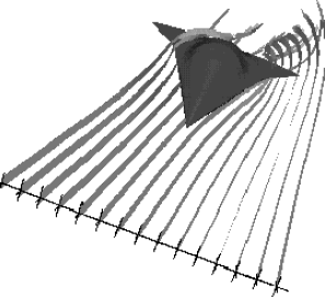
Figure 5.70: Particle Trace Illustration

5.2.10.4. Emitters

A streamline or pathline Particle Trace Part consists of one or more Particle traces originating from points on one or more emitters. Each emitter is capable of emitting a Particle starting at a specified time and continuing to emit Particles at given intervals. When pathlines are generated with emitters emitting at multiple time intervals and these traces are then animated, streaklines are displayed.

Emitters consist of single points, points along a line, points forming a grid in a plane, or points corresponding to the visible nodes of a Part. You can define emitters using the Cursor tool, the Line tool, the Plane tool, or a Part. The traces will be emitted from the visible nodes of the Part (which, for example, will be the surface border nodes if the part element representation is border mode). In fact, if you have a cursor, line or plane tool visible in a flow field, you can right-click the tool and choose Particle Trace to immediately create a particle trace in the flow field using all the default settings.

Emitters can be created using the cursor, line, and plane tools, using existing visible Part nodes, or can be created in a surface restricted mode where the mouse can be used to project points, rakes or nets directly onto the displayed surfaces of the model.

Pathlines, of course, must be drawn forward in time, but streamlines can be drawn forward in time, backward in time, or both. Each Particle trace terminates when either

The Particle trace moves outside the space in which the vector field is defined.
A user-specified time limit is reached.
The massless Particle becomes stationary in a place where the vector field is zero.
The last transient-data time step is reached. (4 applies only to pathlines).

A Particle trace can pass through any point inside an element of the parent Part(s). The vector field at any point is calculated from the shape function of the containing element. Emitter points located outside the elements are ignored when creating Particle traces.

5.2.10.5. Surface-Restricted Traces

A surface-restricted Particle trace is constrained to the surface of the selected Part(s) by using only the tangential component of the velocity. The velocity values for this type of trace can be the velocity at the surface (if nonzero) or at some user specified offset into the velocity field.

5.2.10.6. Interactive Traces

A streamline Particle trace can be updated interactively by entering interactive mode and moving the tool used to create the emitter. When a trace is selected and interactive emitter is turned on, the tool will appear at the location of the emitter. The user then manipulates the tool interactively in the Graphics Window or using the transformations dialog. (This option is not available for surface-restricted Particle traces, traces emitted from a Part nor in Server of Server mode).

5.2.10.7. Integration Method

EnSight creates streamline and pathline Particle traces by integrating the vector field variable over time using a Fourth Order Runge-Kutta method and utilizing a time varying integration step. The integration step is lengthened or shortened depending on the flow field, but you can control the minimum number of integration steps performed in any element as well as other time step controls.

Normally, EnSight will perform the integration using all of the components of the vector. However, it is possible to restrict the integration to a plane by specifying which components of the vector to use. Typical uses of this feature would be to restrict the Particle traces to a clip plane. Surface-restricted Particle traces provide even greater flexibility in restricting a trace to planes or other surfaces.

5.2.10.8. Max # of Segments

A trace will continue until it attempts to leave the flow field or until it reaches the maximum time (Max Time, discussed later) or until it reaches the maximum number of segments. Max Time and maximum number of segments exist because sometimes a trace will continue indefinitely, for example when the trace is caught in a vortex or recirculation area. Each trace has a maximum number of segments. The maximum number of segments in each massless trace is by default 5000 for surface-restricted traces, and 6000 for all other massless trace types. This default can be changed by entering a command line entry (File → Command) into the Command dialog.

Surface restricted:

test: max_skin_segments <value>

All other trace types:

test: max_ptrace_segments <value>

A value of 0 disables the maximum segment check, and for massed particles the value entered is automatically doubled.

5.2.10.9. Lines or Ribbons

Line-type Particle traces consist of bar elements. Ribbons consist of 4-noded quad elements and originate with their end-edge parallel to the Z-axis of the global frame. Then, at each integration step, the leading edge is rotated around the current direction of the path by the same amount the vector field has rotated around the path since the previous time step. Ribbons are not available for surface-restricted Particle traces.

Particle Trace Parts are created on the server, so the Representation-type of the parent Parts has no effect. The algorithm that creates Particle traces initially sets up a cross-referencing map of adjoining elements. Hence, the first Particle trace takes longer to generate than subsequent traces.

If you calculate pathlines, consider calculating as many as possible at a time, since the process can be very time consuming (most of the time is taken in reading time step information). However, the data for the Trace Part is sent to and stored on the Client. Therefore, you cannot label nodes or elements, and some query options may be limited. In such cases, it may be helpful to perform the labeling or query option on the Particle Trace's parent Part(s) instead. Line-type Particle Traces can be parent Parts for Profiles. You can animate the motion of the massless Particles along their Particle traces.

5.2.10.10. Transient Data

By default the emission point is always set to emit the Particles at the current time step. This can be a problem if you have a transient dataset with the current time set at the last time step available. If you compute pathlines from this location, the default emission time will be at the current time (last time step), therefore no pathlines will be generated. To solve this problem you will need to either change the current time, or change the Start Time of the emitter.

The process of creating a streamline or pathline Particle trace is always to specify an emission point (location and time), specify the Part(s) to trace the Particle through and specify which vector variable to integrate. There are quick ways of doing this process which assume that the correct defaults are set, or there are more deliberate ways which give you more control. Particle trace Parts carry only one set of attributes for all of the traces in the Part, therefore it is not possible, for example, to trace some of the emission points forward in time and others backward in time.

Particle trace Parts are different from all other created Parts in that when the parent Parts change (such as at a time step change), the Particle trace Part does not change. This is due to the fact that the Particle trace has been created at a specified time (the emission time), making the Part independent of time (after the trace has been created).

Regular pathline Particle traces can only be computed through a set of parent Parts consisting of model Parts (to avoid the prohibitive cost of updating the non-model part through time). In contrast, streamlines can be computed on non-model parts (because the non-model parts do not have to be updated through time as the streamline calculation proceeds). Surface-restricted Particle traces can be created on model Parts, clip Parts, elevated surface Parts, and developed surface Parts.

If your dataset contains 3D elements, the Particles for regular traces will be traced through 3D element fields only. Surface-restricted traces would have to be used to trace along 2D elements of such a data set.

5.2.10.11. Trace Visibility & Color

Each individual particle trace visibility status and color can be controlled via a right mouse button selection of the particle trace in the graphics window. Coloring individual traces only works if the trace part is a constant color. Right-click an individual trace and select Set trace emission to constant color... to choose a color to set the selected emission. The standard color widget will appear to allow you to select a color. Select Set trace emission to random colors and EnSight will automatically assign a random color to each emission of the particle trace part. To clear the per trace color simply color the part by a constant color. The visibility of each individual trace can be turned invisible by right-clicking on it and selecting Hide this trace emission. Finally, reset all traces to visible using Show all trace emissions.

5.2.10.12. Massed-Particle Traces

A particle trace can be created or updated from a massless-particle trace to a massed-particle trace, or visa-versa. Massed-particle traces are specified via their appended section in the Feature Detailed Editor (Traces) dialog. Massed particle traces use an RK4(5) (Fehlberg) integration algorithm.

Definitions

Motion of a particle as a function of its velocity is defined as

with initial conditions and initial particle position (capital letters denote vectors unless otherwise indicated).

For massless particles, the particle velocity is always identical to the local fluid velocity, .

For massed particles, additional forces acting on them result in a different velocity for the than for the fluid, not equal to .

This particle velocity is determined from a momentum balance for the particle by

or

where

= particle acceleration vector,

= total (particle) force vector,

= gravitational (body) force vector =

= buoyancy (body) force vector =

= pressure (surface) force vector =

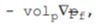
= drag (surface) force(s) vector = - ½ ρ_f a_p c_d | V_r | V_r,

= additional forces vector, here = 0,

given the following definitions.

The underlined definitions below are user specified:

= spherical particle mass =

= volume of particle,

= particle density,

= particle diameter,

= fluid density (scalar or constant),

= gravitational acceleration vector,

= fluid pressure gradient vector, (computed from = fluid pressure scalar variable)

= particle reference area =

= particle velocity vector,

= fluid velocity vector,

= reference velocity vector =

= drag coefficient, typically given as a function of the local relative Re, i.e.

Re = Reynolds number =

= fluid dynamic viscosity (scalar or constant).

Therefore, the total mass balance equation for massed particles may be defined by:

Dividing through by the particle mass m_p yields the following acceleration terms:

Note the following relation in the drag acceleration term:

where: = ballistic parameter or coefficient =

Drag Coefficient

Currently, the following Drag Coefficient () table is provided as the default.

Re << 1 Cd = 24/Re

1 < Re << 500 Cd = 24/Re^0.646

500 < Re << 3e5 Cd = 0.43

3e5 < Re << 2e6 Cd = 3.66E-4 Re^.4275

2e6 < Re Cd = 0.18

This table is also coded as an example for your reference and access via the User-Defined Math Function DragCoefTable1(Re) which is found in

$CEI/ensight242/src/math_functions/drag_coef_table1/libudmf-drag_coef_table1.c

In addition, two other drag coefficient functions are provided for your selection via the User-Defined Math Function facility.

DragCoefPoly(Re) = (a + b Re + c Re² + d/Re )

Where: {a,b,c,d} are polynomial coefficients with default values of {1.,0.,0.,0}, respectively.

DragCoefPower(Re) = (1 + .15 Re^0.687) 24 / Re

Both of these functions are located respectively in:

$CEI/ensight242/src/math_functions/drag_coef_poly/libudmf-drag_coef_poly.cf

$CEI/ensight242/src/math_functions/drag_coef_power/libudmf-drag_coef_power.c

You may also code your own. (See User Defined Math Functions, and/or the Ansys EnSight Interface Manual User Defined Math Functions.)

Rebound Massed Traces (Off a Boundary Wall)

Massed-particle traces can be toggled to rebound off boundary walls. The rebounding massed traces are based on the following derivation. The derivation assumes both the massed particle and boundary wall (or boundary) are both rigid so that there is no deformation of the massed particle or boundary. Also rotational considerations are ignored.

Starting with the initial impact particle velocity (R0)

the tangential friction force opposing the massed particle is given by (R1)

and the normal reaction force is given by (R2)

The tangential friction force is proportional to the normal reaction force by the coefficient of friction μ given by (R3)

Equating R1 to R2, canceling out , and taking into account R3 we have (R4)

Solving for we have (R5)

Now given that in the normal direction the final (reflected) velocity of the massed particle is proportional to the initial (incident) velocity of the massed particle by the coefficient of restitution ε, we have (R6)

which is the final normal component of the rebounding massed-particle velocity. Subbing R6 into R5 and simplifying we have (R7)

which yields the final tangential component of the rebounding massed-particle velocity. Combining these two components (R6 and R7 ) yield the final rebounding particle velocity (R8)

Where:

= the mass of the particle as defined above.

= the friction force tangent to the boundary opposing the particle (therefore the "-" sign on the right hand side of the equation assuming the particle is traveling in the positive direction).

= the normal force on the boundary "opposing" the particle (assuming the normal direction back into the field as positive).

= the tangential component of the particle velocity .

= The tangential component of the incident impacting onto the boundary.

= The tangential component of the reflected bouncing off the boundary.

= The normal component of the particle velocity .

= The normal component of the incident impacting onto the boundary.

= The normal component of the reflected bouncing off the boundary.

= The coefficient of restitution.

= The coefficient of friction.

Particle-Mass Scalar on Boundaries

Information to compute a particle-mass scalar on boundaries () is provided each time massed-particle traces are created. This scalar is found and computed via the New Computed Variables (NCV) functionality.

Massed Particle Scalar(Massed-Particle Traced Part(s))

This scalar creates a massed-particle per element scalar variable for each of the parent parts of the massed-particle traces. This per element variable is the mass of the particle times the sum of the number of times each element is exited by a mass-particle trace.

References

The following references have contributed in part toward the development of the massed-particle algorithm.

Donley, H. Edward "The Drag Force on a Sphere", http:\\www.ma.iup.edu/projects/CalcDEMma/drag/drag.html

Lund, Christoph "Vorgaben fϋr die Berechnung und Visualisierung der Bahnlinien massebehafteter Partikel im Postprozessor EnSight",Volkswagen AG, 27.07.2001. English translation by Kent Misegades.

Fluid Dynamics International, Inc. FIDAP 7.0 Theory Manual", April 1993, pp12-3+

Danby, J.M.A. "Conputing Applications to Differential Equations", Restin Pub. Co., Inc. Restin, VA; 1985

Howard Brady, Rod Cross, Crawford Lindsey "The Physics and Technology of Tennis", Raquet Tech Pub., Solana Beach, CA, 2002

Richard Burden, J. Douglas Faires, Albert C. Reynolds "Numerical Analysis, 2nd Ed.", Prindle, Weber, & Schmidt, Boston, 1978

Paul Tipler "Physics", Worth Pub. Inc.; NY, 1976

Clicking once on the Particle Trace icon (which be default is in the Feature Ribbon) or selecting Particle traces... in the Create menu, opens the Feature Panel for particle trace parts. This editor is used to both create and edit particle trace parts.

Figure 5.71: Particle Trace Icon

Figure 5.72: Feature Panel - Particle Traces - Basic Types

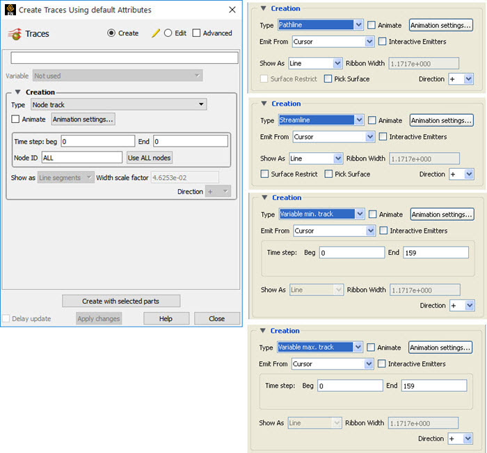
	Create/Edit	Toggles that control whether a new part will be created, or whether you are editing existing part(s). Note: When editing, the changes will be applied to those parts which have the small pencil icon next to them in the Parts list.
	Advanced	Will open additional features for more advance control of the Part.
	Desc	The name of the part to be created or being edited.
Creation
	Type	Opens a pulldown menu for specification of whether Particle trace calculation uses steady-state data (streamlines), transient data (pathlines), or one of the tracking options.
		Node Track	Tracks one (or all) nodes of the selected part(s) through time. Requires node ids and transient geometry or transient displacements.
		Pathline	Traces a massless Particle through a time-varying vector field and so is only available with transient results data and only allowed on model parts. Restriction to Model Parts For even moderately-sized datasets, pathline trace calculations consume significant quantities of CPU and can require substantial I/O as the calculation labors to proceed through time. Restricting this calculation only to model parts avoids the recompute of all the dependent, non model parts through each timestep which can be prohibitively slow.
		Streamline	Traces a massless Particle in a steady-sate vector field (for steady-state data or the current time-step of transient data).
		Variable min track	Tracks the location of the minimum value of the chosen variable through time.
		Variable max track	Tracks the location of the maximum value of the chosen variable through time.
	Emit From	Opens a pulldown menu for the specification of the emitter type.
	Cursor	Creates Particle trace beginning from the position of the Cursor tool.
	Line	Creates Particle traces beginning from the position of the Line tool.
		# Points	This field specifies the number of evenly spaced traces you want to emit from the Line tool.
	Plane	Create Particle traces beginning from the position of the Plane tool.
		# Points	These fields specify the number of traces you want to emit from the Plane tool in the X and Y axes of the tool.
	Part	Creates particle traces beginning from visible nodes of the Part specified by the Part ID Number field.
		Part ID	This field specifies the Part you wish to use as an emitter for the creation of a particle trace. The Part ID number for a Part is found in the Parts list. Limitation: once create a trace using a Part ID, this ID can no longer be changed, nor can you change the emitter type.
		Number of	This field specifies the number of emitters desired. They will be randomly selected from
		Emitters	the visible nodes of the part. (see Created Parts)
	File	Creates particle traces from the locations specified in an external file. (see EnSight Particle Emitter File Format)
	Time step: Beg, End	For Tracking types, specifies the beginning and ending time steps to use for the track.
	Node ID	Field for specifying the desired node id of a Node Track. Note: A single node id can be specified to track a single node, or ALL can be specified to track all nodes of the selected part(s).
	Use ALL nodes	Clicking this button sets the value in the Node ID field to ALL.
	Show As	Opens the pull-down menu for specification of trace representation for streamline and pathline traces.
		Line	Depicts the trace as a line.
		Ribbon	Depicts trace as if it were a ribbon. The ribbon width is a specified fixed value, while the twisting is determined by the rotation of the flow about the path of the trace at any particular point on the trace.
		Square Tubes	Depicts trace as if it were a square tube. The tube width is a specified fixed value, while the twisting is determined by the rotation of the flow about the path of the trace at any particular point on the trace.
		Tubes	Depicts trace as if it were a round tube. The tube width is a specified fixed value. There is no indication of twisting when using tubes.
	Ribbon Width	This field only applies when Ribbon representation is chosen. Larger values in this field produce wider ribbons. Only available for streamlines and pathlines.
	Surface Restrict	Toggles on/off surface restricted feature for streamlines. The streamline will be constrained to stay on the surface of the selected Part(s) by using only the tangential component of velocity. Be sure to use the Pick Surface feature in locating the emitter for a surface restricted particle trace to ensure that the emitter is located on the surface of a Part
	Pick Surface	Toggles on/off the feature which allows you to place the trace emitter at a point on a surface directly below the mouse pointer by clicking the left mouse button.
	Direction	Trace the Particle in positive time, meaning to trace with the vector field, or trace the Particle in negative time, meaning to trace the Particle upstream. Option only applies to streamlines. Pathlines must be traced in + time.
		(+)	Positive time option traces Particle(s) forward in time. (This is the only option for pathlines.)
		(-)	Negative time option traces Particle(s) backward in time.
		(+/-)	Positive/Negative time option traces Particle(s) both forward and backward in time.
	Animate Toggle	Toggles on/off the animation of the motion of the Particles along the traces. In addition to creating Particle traces based on vector variables, EnSight can also animate the motion of the Particles along the Particle traces. To distinguish them from discrete Particles, we call Particles moving along Particle traces tracers.
		At any instant, each tracer consists of a portion of a Particle trace displayed with attributes you specify separately from the attributes of the Particle trace. EnSight animates each tracer by updating which portion of the Particle trace is currently displayed. You specify the length of each tracer as a time value, so the tracer's length varies dynamically as it moves down the Particle trace (faster moving tracers are longer). This option can add tremendously to the understanding of the flow field since relative speed can be determined. EnSight provides control over how the tracer looks and acts. You can animate one, some, or all of the Particle traces you have created, but they are all animated in the one way you specify. To help you get started, at the click of a button EnSight will suggest time-specification values based on the Particle traces you have selected to animate. You can specify the line width of the tracer, and choose to color it with a constant color or the same calculated color used to color the Particle trace. You can also display a spherical head on the leading-end of the tracer, and dynamically size the head according to any active variable. You control the speed of the motion and have the option to display multiple tracers on the same Particle trace separated by a time interval. Hence, you can choose to view rapid-fire pulses, slow moving noodles, or something in between. For steady-state Particle traces (streamlines), time is the integration time with the emitters located at time zero. For transient Particle traces (pathlines), you have the option to synchronize the animation time to the solution time. The choice of whether a Particle trace is a streamline or a pathline is made when you create the Particle trace. You do not have to animate the entire Particle trace. You can specify where you want the animation to start with a time value corresponding to a distance down the Particle trace from the emitter, and where you want the animation to stop with a time value corresponding to a distance farther down the Particle trace. Tracers on all animated Particle traces are synchronized. If you combine Particle trace animation with flipbook animation or keyframe animation, the animation time values are automatically synchronized if you toggle-on Sync To Transient in the Trace Animation Settings dialog.
Animation settings...	Opens the Trace Animation Settings dialog. Figure 5.73: Trace Animation Settings Dialog
	Color By	Opens a pulldown menu for selection of method by which to color the tracers.
		Constant	Displays tracers in the constant color specified in this dialog.
		Mix...	Opens the Color Selector dialog (see Auxiliary Geometry).
		R,G,B	Fields allow specification of constant color.
		Trace Color	Displays tracers in the same color as the Particle Trace Part from which they originate.
	Line Width	Specification of displayed width (in pixels) of tracers. Note: Line Width specification may not be available on some workstation platforms.
	Start Time	Specification of how far down each Particle trace to begin displaying tracers. A Particle trace is made up of line segments. Each segment that makes up a Particle trace has an associated time value. The start time indicates where on the Particle trace the tracers will begin animation.
	Tracer Time (Length)	Specification of length of tracers which varies as the tracer speed varies along the Particle trace. The Particle Time Length parameter scales the length of all tracers at all times.
	Tracer Delta (Speed)	Specification of how fast tracers move. Longer times result in faster moving tracers. This parameter is not applicable when using Sync To Transient and displaying transient data through flipbook or keyframe animation.
	Sync to Transient	Toggles on/off synchronization of tracer position to solution time of transient data. When toggled-on, and transient data is in use (i.e. solution time, flipbook or keyframe animations), each tracer is displayed with its leading-end at the correct location along the Particle trace for the current solution time. Traces only move forward in time so cycling through transient data is not applicable here.
	Max Time Toggle	Toggles on/off maximum lifetime for all tracers. If toggled-off, tracers continue to end of Particle trace. If toggled-on, each tracer stops after moving down the Particle trace for a distance corresponding to the specified Max Time (or until one of the other conditions that stop a tracer occurs).
	Max Time	Field specifies lifetime of all tracers when Set Max Time is toggled-on.
	Multiple Pulses Toggle	Toggles on/off multiple emission of tracers. When toggled-off, a single tracer for each Particle trace appears at the specified Start time. When toggled-on, additional tracers appear after each specified Pulse Interval. Not applicable to pathlines.
	Pulse Interval	Field specifies time delay between tracers. Not applicable when Multiple Pulses is toggled-off.
Tracer Head Representation
	Type	Opens a pulldown menu for selection of type of head for each tracer.
		None	Specifies that no head will appear.
		Spheres	Specifies that a sphere will appear on the leading end of the tracer.
		Scale	Specification of scaling factor for head size. Values between 0 and 1 reduce the size, factors greater than one enlarge the size. Not applicable when Head Type is None.
		Size By	Opens a pulldown menu for the selection of variable-type to use to size each tracer's head. If you select a variable, the head size is determined by multiplying the Scale factor times the variable value, which will vary depending on the location of the tracer. Not applicable when Head Type is None. Constant Sizes head using just the Scale factor value. Scalar Sizes head using a scalar variable. Vector Mag Sizes head using magnitude a vector variable. Vector X Sizes head using X-component of a vector variable. Vector Y Sizes head using Y-component of a vector variable. Vector Z Sizes head using Z-component of a vector variable. Variable Selection of variable to use to size the tracer heads. Not applicable when Type is None or Size By is Constant.
	Get Defaults	Click to set time-value specifications in this dialog to values suggested by EnSight based upon the characteristics of the selected Particle traces.
		See Also: Animate Particle Traces

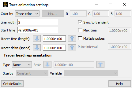
Troubleshooting Animated Particle Traces

Problem	Probable Causes	Solutions
No motion. Can't see any tracers.	No Particle traces selected to animate.	Select the traces you wish to animate in the list at the top of the Animated Trace Setup dialog.
	Tracers colored same as Particle traces and have same line width.	Change Color By or Line Width.
	Animate Traces not toggled-on.	Toggle Animate on in the Feature Panel.
	Start Time → maximum Particle trace time for all traces selected.	Change settings in the Trace Animation Settings dialog.
	Delta Time (Speed) set too high.	Change settings in the Trace Animation Settings dialog.
	Particle Time (Length) set too small.	Change settings in the Trace Animation Settings dialog.
Motion too fast.	Delta Time (Speed) set too high.	Change settings in the Trace Animation Settings dialog.
Can't get multiple pulses at same time.	Pulse interval too high.	Decrease to have pulses start closer together.
Have one big tracer, no pulses.	Pulse interval too small, pulses start right after each other with no separation.	Increase the interval.

Interactive Emitter	Toggles on/off interactive Particle tracing. Manipulation of the Cursor, Line or Plane tool will cause the Particle trace to be recreated at the new location and updated in the Graphics Window. When manipulation of the tool stops, the Particle trace and any Parts that are dependent on it will be updated. (Only available for non-surface-restricted streamlines).
	Figure 5.74: Feature Panel - Particle Traces - Advanced
Scaling
XYZ	For vector variables, in advanced mode, specify vector components used in creating the particle traces. Not applicable to scalar variables. Are according to the reference frame of the parent part. Letters labeling dialog data entry fields depend on type of the reference frame (Rectangular, Spherical, or Cylindrical). If all components are 0.0, the vector magnitude will be used. But, if any of these scaling factors is non-zero, the variable value will be computed as .
Creation (Additional)
Variable offset	This field specifies the distance into the flow field at which velocity (and other variables) are to be sampled for the surface restricted trace(s). If velocity values are present at the surface, this offset can be set to zero.
Display offset	This field specifies the normal distance away from a surface to display the surface restricted traces. A positive value moves the traces away from the surface in the direction of the surface normal. Note: There is a hardware offset that will apply to contours, vector arrows, separation/attachment lines, and surface restricted particle traces that can be turned on or off in the View portion of Edit → Preferences. This preference (Use graphics hardware to offset line objects...) is on by default and generally gives good images for everything except move/draw printing. This hardware offset differs from the display offset in that it is in the direction perpendicular to the computer screen monitor (Z-buffer). Therefore, for viewing, you may generally leave the display offset at zero. But for printing, a non-zero value may become necessary so the traces print cleanly.
Arrows	Controls whether the flow direction is indicated with arrows.
	None	option displays arrows as lines without tips.
	Cone	arrows have a tip composed of a 3D cone. Good for both 2D and 3D fields.
	Normal	arrows have two short line tips, similar to the way many people draw arrows by hand. The tip will lie in the X-Y, X-Z, or Y-Z plane depending on the relative magnitudes of the X, Y, and Z components of each individual vector. Suggested for 2D problems.
	Triangles	arrows have a tip composed of two intersecting triangles in the two dominant planes. Good for both 2D and 3D fields.
# of Arrows	Controls density of arrows. The trace with the longest dwell time will have this number of arrowheads, and the other traces will get a number that corresponds to their dwell time.
Arrow Size	Scaling size of Arrowheads.
Emitter Information
Emitters List	This section shows a list of all emitters created for the currently selected Particle Trace Part.
Add Emitter	Adds an emitter of the type specified by Emit From to the currently selected Particle Trace Part.
Delete Emitter	Deletes the emitter selected in the Emitters List from the selected Particle Trace Part.
Emit at current time	Toggle on to set the emitter to the current time.
Total Time Limit	This field specifies the maximum residence time of the trace, meaning the difference in time between emission time and trace termination time. For pathlines the traces will also be terminated once the end solution time (as defined in the Time Control Panel, see Solution Time) is processed. Note: This limit is applied to each direction (+/-) independently.
Set to default	This button sets the Total Time Limit field to a reasonable default value using the vector value and the geometry size.
Emission Time Start	This field specifies the solution time at which to begin Particle emission. Enter value between beginning and ending time available.
Time Delta	This field specifies the time interval between emissions of Particles from the emitters. If 0, only one set of emissions will occur at start time
Time Step Determination	The entries in this section allow the user to control the number and size of the integration steps used to create traces.
Min Steps	This field is used to specify the minimum number of integration steps to perform in each element.
Min Angle	If angle between two successive line segments of the Particle trace is less than this value EnSight will double the integration step.
Max Angle	If angle between two successive line segments of the Particle trace is greater than this value EnSight will half the integration step.
Rot Angle	If the change in rotation angle at two successive points of the Particle trace is greater than this value, the integration step is halved.
Compute using Periodicity	Toggles on/off the periodicity feature. The default is OFF. If this toggle is ON and the parent part has visual symmetry (see Set Symmetry) set to rotational, then the particle tracer will attempt to trace the particle path out of a symmetry plane and back into the other symmetry plane. This results in a somewhat confusing trace unless you turn on instances of symmetry of the parent part and of the particle trace part, to see clearly the traces as they move through the symmetry instances. For usage details, see Create Particle Traces.
Massed Particle Attributes	Opens the massed-particle attributes area.
Use massed particles	Toggles on/off the massed-particle traces feature. The default is OFF
	Note: Some dependent parameters are duplicated under multiple tabs for reference convenience, i.e. Gravity under Gravity and Buoyancy tabs. These parameters are updated under all applicable tabs when changed under a particular tab.

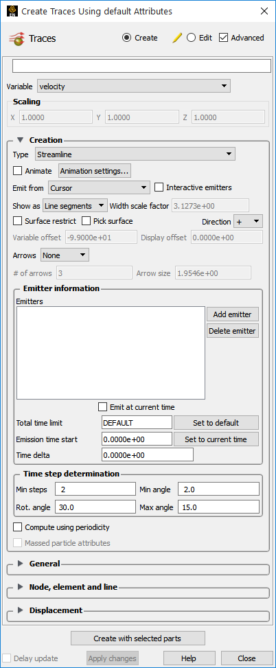
Drag term tab	Showing dependent parameters for drag acceleration term (default selection)
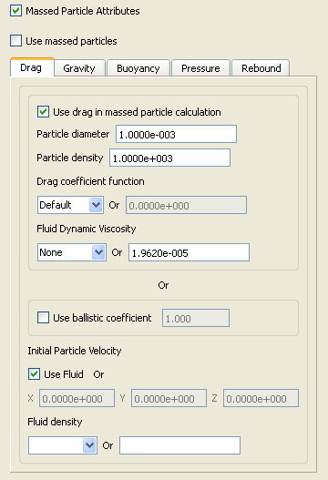Use drag in massed particle calculation	Toggles on/off the inclusion of the drag term in the massed-particle computation. The default is ON
Particle diameter	This field specifies the diameter of all particles. The default is 1.e-3.
Particle density	This field specifies the density value of all particles. The default is 1.e+3.
Drag coefficient function	This field specifies the drag coefficient function to be called each time the drag coefficient is calculated. This function defaults to Default which essentially defaults to the table described above. Other functions may be accessed via the User-Defined Math Function facility, i.e. DragCoefTable1(Re) (same as default), DragCoefPoly(Re), DragCoefPower(Re). All functions must take the Reynolds Number as their only argument. This parameter only works with the drag term.
Or
	This field specifies the drag coefficient value to be used in the computation if None is specified as the variable name. The default value is 0. This parameter only works with the drag term.
Fluid dynamic viscosity	This field specifies the fluid dynamic viscosity variable to be used in the massed-particle computation. The default is None.
Or
	This field specifies the fluid dynamic viscosity value to be used in the computation if None is specified as the variable name. The default value is 1.9620e-5. This parameter only works with the drag term.
Use ballistic coefficient	Toggles on/off the use of the ballistic coefficient value () in place of the above drag parameters which are greyed-out, i.e. particle diameter and density (used in mp and ap), and drag coefficient and fluid dynamic viscosity (used in cd). The default toggle is OFF. When toggled ON, the default value is 1.
Initial particle velocity	Determines what initial velocity to use for all the particle emitters. The default is Use fluid ON. This parameter only works with the drag term.
Use fluid	Toggles on/off whether all particle emitters should use the fluid velocity at their corresponding locations. The default is ON.
Or X, Y, Z	These fields specify the initial velocity components of all particle emitters. Their default is <0., 0., 0.>.
Fluid density	This field specifies the fluid density variable to be used in the massed-particle computation. The default is None. This parameter only works with the buoyancy term.
Or
	This field specifies the fluid density value to be used in the computation if None is specified as the variable name. The default value is 1.
Gravity term tab	Showing dependent parameters for gravity acceleration term
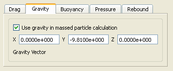Use gravity in massed particle calculation	Toggles on/off the inclusion of the gravity term in the massed-particle computation. The default is ON
Gravity vector	These fields specify the gravity vector to be applied in the massed-particle computation. The default gravity components are <0., -9.81, 0.>. This parameter only works with the gravity and buoyancy terms.

Buoyancy term tab	Showing dependent parameters for buoyancy acceleration term
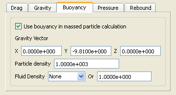Use buoyancy in massed particle calculation	Toggles on/off the inclusion of the buoyancy term in the massed-particle computation. The default is ON
Gravity vector	These fields specify the gravity vector to be applied in the massed-particle computation. The default gravity components are <0., -9.81, 0.>. This parameter only works with the gravity and buoyancy terms.
Particle density	This field specifies the density value of all particles. The default is 1.e+3.
Fluid density	This field specifies the fluid density variable to be used in the massed-particle computation. The default is None. This parameter only works with the buoyancy term.
Or
	This field specifies the fluid density value to be used in the computation if None is specified as the variable name. The default value is 1.

Pressure gradient term tab	Showing dependent parameters for pressure-gradient acceleration term
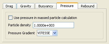Use pressure in massed particle calculation	Toggles on/off the inclusion of the pressure-gradient term in the massed-particle computation. The default is OFF
Particle density	This field specifies the density value of all particles. The default is 1.e+3.
Pressure gradient	This field specifies the fluid pressure gradient variable to be used in the massed-particle computation. The default is None. This parameter only works with the pressure force term.

Rebound term tab	Showing dependent parameters for allowing rebound of massed traces
Use rebound in massed particle calculation	Toggles on/off the inclusion of rebound parameters to account for coefficient of restitution and friction effects when massed traces contact boundaries. The default is OFF Note: Rebound requires an active acceleration term, i.e. Drag, Gravity, Buoyancy, and/or Pressure.
Coefficient of restitution	This field specifies the coefficient of restitution value to be used for all massed trace computations. The default value is 0. (no restitution - no rebound). The typical range for this value is 0. to 1. (The value of 1 being full restitution, or a perfect elastic bounce off the wall where the angle of reflection off the boundary into the field is equal to the angle of incidence into the wall from the field.) This value is combined with the coefficient of friction to determine the final rebound of the massed particle off the boundary wall.
Coefficient of friction	This field specifies the coefficient of friction value of the boundary to be used for all massed trace computations. The default value is 0. (no friction). The typical range for this is 0. to <1. This value is combined with the coefficient of restitution to determine the final rebound of the massed particle off the boundary wall.
Fraction of initial impact velocity	This field specifies a fraction of the initial impact velocity (magnitude) value to be used as a stopping criteria for a rebounding massed particle. The default is .01.
Maximum number of wall hits	This field specifies the maximum number of wall hits (per massed particle) value to be used as a stopping criteria for a rebounding massed particle. The default value is 10 hits.

Create with selected parts	Creates Material part using the selected Part(s) in the Parts list.
Delay update	Checking this box will cause EnSight to not apply any changes made until you hit the Apply Changes button. When not checked, the changes are applied as you make them.
Apply Changes	Applies any changes made. Only active when Delay update is on.

See Feature Panel Turndowns Common To All Part Types for a detailed discussion of the remaining Feature Panel turn-down sections which are the same for all Parts.

See Create Particle Traces

Troubleshooting Particle Traces

Problem	Probable Causes	Solutions
Particle Trace Part is empty.	Velocity is zero.	Change time steps or change location of emitters.
	Emitter points are outside of flow field.	Change location for emitter points.
	Dataset is 3D and parent Parts are 2D, or dataset is 2D and parent Parts are not planar.	Change parent Parts.
	The created variable selected does not exist for the parent Part(s)	Recreate the variable for the parent Part(s) selected
	The emitter part is non visual and has no visible nodes	Make the emitter part element representation 3D Border 2D Full to obtain visible nodes
Streamline is OK, but pathline is empty.	Creating pathline with the emitter emitting at the last time step.	Modify emitter time for the emitter groups.
Particle trace terminates prematurely	Velocity has gone to zero.	None
	Particle has been traced out of the flow field.	None
	Stopping point is at the boundary between two Parts.	Change the parent Parts for the Particle trace to include neighbor Part.
	Particle getting lost and EnSight's search algorithm failing.	Call Ansys hotline support.
	Total Time Limit reached.	Change Total Time Limit.
Particle trace exists, then is removed after deleting Parts.	The parent Part for the Particle trace was deleted.	None
Particle trace creation requested, but Particles don't come back.	Requested a large number of Particle traces and/or doing pathlines in large transient dataset.	Be patient.
	Particles are stuck in a recirculation area.	Process will finish when Total Time Limit is reached. Consider terminating job and starting over with a smaller Total Time Limit.
Interactive tracing is slow.	The size of the model and density of the mesh will affect the performance of an interactive trace.	If you can, run on a faster, larger memory workstation. Also, limit if possible the area of interest by cutting the mesh into pieces with the Cut & Split Part editing operation.
Interactive trace does not enter the next Part	Interactive tracing is only done through the Part the emitter resides in.	When you let go of the emitter the full trace will be shown
Surface restricted Particle trace does not appear	Zero velocity at chosen variable offset	Select a Variable offset distance that will give nonzero velocity
	Display offset causing trace to be on opposite side of a surface (hidden surface on)	Change sign of the Display offset. Note: Offset is in the direction of the surface element normal.
	Emitter does not lie on the surface of selected Parts	Create emitters that lie on the surface
Surface Restricted particle trace does not print well	See Display Offset discussion above	Enter a non-zero display offset.

5.2.11. Point Parts

Point parts are composed only of nodes. They can be created by reading an external file containing the xyz coordinates of the nodes, and/or by placing the cursor tool at desired locations and adding nodes. This feature can be used to essentially place probes in the model at particular locations. It can also be used to create parts that can be meshed with the 2D or 3D meshing capability within EnSight.

Clicking once on the Point parts icon (if you have customized the Feature Ribbon to have it visible) or selecting Point parts... in the Create menu, opens the Feature Panel for Point parts. This editor is used to both create and edit Point parts.

Figure 5.75: Point Parts Icon

Figure 5.76: Feature Panel - Point Parts

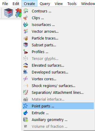
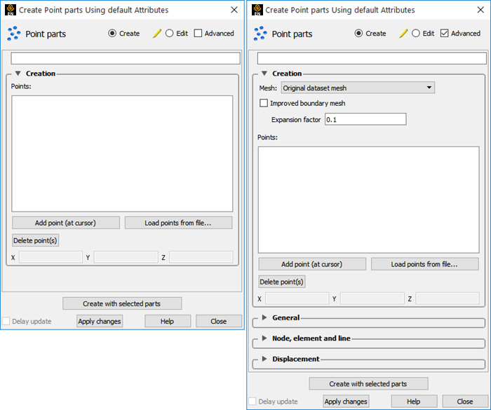
Create/Edit	Toggle controls whether a new part will be created, or whether you are editing existing part(s). Note: When editing, the changes will be applied to those parts which have the small pencil icon next to them in the Parts list.
Advanced	Will open additional features for more advance control of the Part.
Desc	The name of the part to be created or being edited.
Creation
Mesh	Opens pulldown menu for selection of part meshing to use. 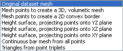The default is to use the element connectivities described in the model data file(s). But a remeshing can be done, utilizing the `QHull` library. This library can compute the convex hull of point data, a 2D meshing. And since the convex hull of a 3D dataset lifted into 4 dimensional space turns out to be the volumetric tetrahedralization of the 3D data, it can be used to do a 3D meshing as well. Note: This remeshing can take considerable memory and processing - so it must be used with that in mind. Also, the worst case for `QHull` is a large number of co-planar points. In the higher-dimensional lifting step, the planarity adds a singularity that is difficult to work around. Using bounding boxes and planar projections can help. Accordingly, several options exist, which can be used if your data exhibits problematic characteristics. The pulldown menu options are:
	Original dataset mesh	The nodes and elements described in the model data file(s) is used. No remeshing is done. This is the default.
	Mesh points to create a 3D, volumetric mesh	The original element connectivities will be replaced with a volumetric meshing of the nodes of the part, to produce tetrahedral elements.
	Mesh points to create a 2D convex border	The original element connectivities will be replaced with a convex hull meshing of the nodes of the part, to produce triangle elements.
	Height surface, projecting points onto YZ plane	The original element connectivities will be replaced. The nodes of the part will be projected to the YZ plane and then triangulated in 2D. The resulting triangle element connectivities will be used with the original node data.
	Height surface, projecting points onto XZ plane	The original element connectivities will be replaced. The nodes of the part will be projected to the XZ plane and then triangulated in 2D. The resulting triangle element connectivities will be used with the original node data.
	Height surface, projecting points onto XY plane	The original element connectivities will be replaced. The nodes of the part will be projected to the XY plane and then triangulated in 2D. The resulting triangle element connectivities will be used with the original node data. Note: There are a few formats that will not allow you to return to the input dataset elements once you have meshed the part. Most do. For these few (ABAQUS fil, Ansys, ESTET, Ansys FIDAP Neutral, Fluent Universal, and N3S), you can change between the 2D and 3D meshing options, but you need to delete the part and reload it, if you desire the part back to the input elements.
Improved boundary mesh	If one of the remeshing options is used, this toggle will employ a common trick that often helps with the co-planar points problem described above. The trick consists of adding 8 points (one at each corner of the bounding region) to the other points. This basically embeds the original points inside of an 8-point box. Then compute the volume tets and remove any tets connected to the non-original box points. Note: An offset can be used for the bounding region to ensure that the bounding region is not collapsed to 2D space (see Expansion factor below).
Expansion factor	When adding the 8 points for the Improved boundary mesh trick above, an offset can be used to expand the bounding region in all directions. This is that offset, or expansion value.
Points	The list of points that will be used to create a point part, or that are in an already created point part. When points are added, they will show up in this list. Use this list to select points for modification or deletion
Add point (at cursor)	Adds a point (at the xyz location of the cursor) to the list of points.
Load points from file...	Brings up the file selection dialog, so a file which contains the xyz locations of points, can be selected. Points in the file will be added to the Points list. (see Point Part File Format).
Delete point(s)	Deletes any points selected in the Points list.
XYZ	Shows the xyz coordinates of a selected point. Allows for editing of the values.
Create with selected parts	Creates a Point part using the selected Part(s) in the Parts list.
Delay update	Checking this box will cause EnSight to not apply any changes made until you hit the Apply Changes button. When not checked, the changes are applied as you make them.
Apply Changes	Applies any changes made. Only active when Delay update is on.

See Feature Panel Turndowns Common To All Part Types for a detailed discussion of the remaining Feature Panel turn-down sections which are the same for all Parts.

See Use Point Parts.

5.2.12. Profile Parts

Profiles visualize values of a variable along a line with a plot projecting away from the line. Projectors are parallel to a plane, but not necessarily in a plane. Hence, Profile can follow the line.

You can scale and offset projectors. The positive direction is set as the From Point as the origin point of the Plane Tool (away from center point is positive). Consider a base-line (not necessarily straight) along which the value of a variable is known. Moving along this base-line, you can plot the value of the variable on an axis whose origin moves along the base-line and whose orientation varies so that it is always both perpendicular to the base-line and parallel to a specified plane (but not necessarily parallel to a line, enabling the plot-line to follow the curve of the base-line in one dimension). A surface joining the base-line to the plot-line is called a profile.

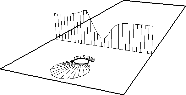
The parent Part of a Profile-Part can be a 1D-Clip Line, a Contour, a Particle Trace, or a model Part consisting of a chain of bar elements. From each node of the parent Part, EnSight draws a projector whose length is proportional to the value of the variable at the node, and whose orientation makes it:

Parallel to a specified plane
Pointing in a direction corresponding to the sign of the variable's value at the node (with the negative-direction determined by the location of a specified point)
Perpendicular to the base-line elements adjoining the node, or, if the base-line bends at the node, oriented so that its projection into the plane defined by the base-line elements will bisect the angle formed by the base-line elements

The outer-end of each projector is connected to those of its neighbors, forming a series of four-sided polygons and hence a surface.

The appearance of the profile depends greatly on the position of the location of the plane tool origin (From Point) and the orientation of the specified plane, which you can specify numerically or with the Plane tool. EnSight calculates the projectors using the vector cross-product of the specified-plane's normal (the Z-axis) and each parent Part element, therefore you should orient the plane so that its normal is not parallel to the parent Part elements.

The projector length is calculated by adding to the variable's value an Offset value, then multiplying the sum by a Scaling value. Adding the Offset enables you to shift the zero location of the projectors, which might be useful if you wanted to make all the projectors have the same sign. An offset performs a shift, but does not change the shape of the resulting profile. The Scaling factor changes the displayed size of the profile, a stretching type of action. EnSight will provide default values for both factors based on the variable's values at the parent Part's nodes.

Clicking once on the Profiles icon (if you have customized the Feature Ribbon to have it visible) or selecting Profiles... in the Create menu, opens the Feature Panel for Profile parts. This editor is used to both create and edit Profile parts.

Figure 5.77: Profile Icon

Figure 5.78: Feature Panel - Profiles

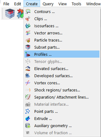
Create/Edit	Toggles that control whether a new part will be created, or whether you are editing existing part(s). Note: When editing, the changes will be applied to those parts which have the small pencil icon next to them in the Parts list.
Advanced	Will open additional features for more advance control of the Part.
Desc	The name of the part to be created or being edited.
Variable	Choose the variable to use for creating the profile part from the pulldown.
Scaling
XYZ	For vector variables, in advanced mode, specify vector components used in creating the profiles. Not applicable to scalar variables. Scaling is in the reference frame of the parent part. Letters labeling dialog data entry fields depend on type of the reference frame (Rectangular, Spherical, or Cylindrical). If all components are 0.0, the vector magnitude will be used. But, if any of these scaling factors is non-zero, the variable value will be computed as .
Creation
Scale Factor	This field specifies the scaling for magnitude of the projector. The Scale Factor is multiplied times the value of the variable. Values larger than one increase the size and values smaller than one decrease the size.
Offset	The value specified in this field is added to the variable values before the Scale Factor is applied to change the magnitude of projectors. Default offset is magnitude of most-negative projector (making them all positive). Has the effect of shifting the plot, but does not change the plot shape.
Set to default	Click to set Scale Factor and Offset values to the calculated defaults based on the variable values for the parent Part.
Show Orientation Tool	Causes the Plane Tool to become visible in the Graphics Window at the location specified
Update Orientation	Recreates the Profile Part at the current location and orientation of the Plane Tool.
Orientation Plane
Pos XYZ	Specification of the location, orientation, and size of the Plane Clip using the coordinates (in the Parts reference frame) of three corner points, as follows: C1 Corner 1 is corner located in negative-X negative-Y quadrant C2 Corner 2 is corner located in positive-X negative-Y quadrant C3 Corner 3 is corner located in positive-X positive-Y quadrant
Set Tool Coords	Will reposition the Plane Tool to the position specified in C1, C2, and C3.
Get Tool Coords	Will update the C1, C2, and C3 fields to reflect the current position of the Plane Tool.
Create with selected parts	Creates a Profile part using the selected Part(s) in the Parts list.
Delay update	Checking this box will cause EnSight to not apply any changes made until you hit the Apply Changes button. When not checked, the changes are applied as you make them.
Apply Changes	Applies any changes made. Only active when Delay update is on.

See Feature Panel Turndowns Common To All Part Types for a detailed discussion of the remaining Feature Panel turn-down sections which are the same for all Parts.

See Create Profile Plots.

Troubleshooting Profiles

Problem	Probable Causes	Solutions
The entire profile is not projected the direction you want.	The Plane is not oriented correctly.	Turn on the Plane tool so you can see its orientation. The projectors will be parallel to this plane, so adjust its orientation.
The entire profile is not projected the direction you want.	The From Point (plane tool origin) is not in a good location	Turn on the Plane tool so you can see the location of the center of the plane. Positive projectors will go away from this point, negative towards.
Portions of the profile appear to be projected in the wrong direction.	The From Point is not in a good location.	Turn on the Plane tool so you can see the location of the center of the plane. Positive projectors will go away from this point, negative towards.
	The normal to the Plane is parallel to some of the elements of the parent Part.	Turn on the Plane tool so you can see its orientation. Try to make sure the Z axis of the Plane tool does not lie parallel to any portions of the parent Part.
	The Parent Part does not contain elements which are consistently ordered	None

5.2.13. Separation/Attachment Line Parts

Separation and Attachment Lines exist on 2D surfaces and help visualize areas where flow abruptly leaves or returns to the 2D surface in 3D flow fields. These lines are topologically significant curves on the 2D surface where flow converges and then separates (separation lines) from the surface into the 3D flow field, and where flow attaches and then diverges (attachment lines) to the surface from the 3D flow field.

These line segments can be used as emitters for ribbon traces to help visualize flow interaction from the 2D surface into the 3D field, or displayed along with surface-restricted traces to help visualize the topology of the 2D surface.

EnSight creates separation and attachment lines as two distinct parts so that each may be assigned their own attributes. Although both are updated computationally when changes are made to either one via the Feature Panel.

Separation/Attachment lines can be created on any 2D part, whether it is a boundary surface or internal surface to a 3D flow field. These lines can also be created on 3D flow field parts. However, computation of the separation/attachment lines is restricted to only the boundary surfaces of the 3D flow field.

5.2.13.1. Velocity Gradient Tensor

EnSight creates separation and attachment lines from the velocity gradient tensor of the 3D flow field part. EnSight automatically pre-computes the velocity gradient tensor for all 3D model parts prior to creating the separation and attachment lines. These values are then mapped to any corresponding 2D model part, or inherited by any created part.

Since this variable is automatically created, all subsequent 3D model parts created will also have this tensor variable computed.

Note: The velocity gradient tensor variable will continue to be created and updated for all 3D model parts until it is deactivated.

This tensor variable behaves like any other created tensor variable, and may be deactivated in the Variables List.

5.2.13.2. Thresholding

Separation/Attachment lines may be filtered out according to the settings of a threshold variable, value, and relational operator. Most active variables can be used as threshold variables. Thresholding was implemented to help you to filter-out, or view portions of the line segments according to variable values.

When separation and attachment line parts are Created/Updated, the scalar variable fx_sep_att_strength is created to help you threshold unwanted core segments according to these scalar values.

Note: This scalar variable is currently set to the vorticity magnitude scalar, until a better thresholding variable can be identified.

Since it has been observed that the current implementation of this algorithm may produce additional lines that are not separation or attachment lines, the need for a filtering mechanism that filters out segments according to different variables arose and had been provided via thresholding options.

5.2.13.3. Algorithms

Currently, separation and attachment lines are calculated according to the phase-plane algorithm presented by Kenwright (see References below). This algorithm detects both closed and open separation. Closed separation lines originate and terminate at critical points, whereas open separation lines do not need to start or end at critical points.

This technique is linear and nodal. That is, 2D elements are decomposed into triangles, and then closed-form equations are solved to determine the velocity gradient tensor values for eigen-analysis at the nodes. Also, any variables with values at element centers are averaged to element nodes before processing.

5.2.13.4. References

Refer to the following references for more detailed explanations of pertinent concepts and algorithms.

J. Helman, L. Hesselink"Visualizing Vector Field Topology in Fluid Flows",IEEE CG&A, May 1991

D. Kenwright, "Automatic Detection of Open and Closed Separation and Attachment Lines", IEEE Visualization '98, 1998, pp. 151-158

R. Haimes and D. Kenwright, "On the Velocity Gradient Tensor and Fluid Feature Extraction", AIAA-99-88, Jan. 1999, pp. 315-4

S. Kenwright, C. Henze, C. Levit, "Feature Extraction of Separations and Attachment Liens", IEEE TVCG, Apr.-Jun. 1999, pp. 135-144

R. Peikert, M. Roth, "The 'Parallel Vectors' Operator - a vector field visualization primitive", IEEE Visualization ' 99, 1999

D. Kenwright, T. Sandstrom, GEL, NASA Ames Research Center, 1999

R. Haimes, D. Kenwright, The Fluid Extraction Tool Kit,Massachusetts Institute of Technology, 2000

5.2.13.5. Access

Clicking once on the Separation and Attachment lines icon (if you have customized the Feature Ribbon to have it visible) or selecting Separation Attachment lines... in the Create menu, opens the Feature Panel for Sep./Att. line parts. This editor is used to both create and edit Separation and Attachment line parts.

Figure 5.79: Feature Panel - Separation/Attachment Lines

Create/Edit	Toggles that control whether a new part will be created, or whether you are editing existing part(s). Note: When editing, the changes will be applied to those parts which have the small pencil icon next to them in the Parts list.
Advanced	Will open additional features for more advance control of the Part.
Desc	The name of the part to be created or being edited.
Creation
Define Sep/Attach Variables...	Opens the Sep/Attach Line Variable Settings dialog which allows you to identify and set the dependent variables used in computing separation and attachment lines. This dialog has a list of current accessible variables from which to choose. Immediately below is a list of dependent variables with corresponding text field and SET button. The variable name in the list is tied to a dependent variable below by first highlighting a listed variable, and then clicking the corresponding dependent variable's SET button, which inserts the listed variable into its corresponding text field. You must specify either `Density` and `Momentum` (which permits velocity to be computed on the fly), or just `Velocity`. A default constant value is supplied for the Ratio of Specific Heats which can be changed or specified by a scalar variable name. Clicking OK activates all specified dependent variables and closes the dialog.
Method	Opens a pop-up dialog for the specification of which type of method, to use to compute the separation and attachment lines on the 2D surface. There is currently only one option:
	Phase Plane	Scheme that uses eigen-analysis on the velocity gradient tensor along with phase plane analysis to compute the separation and attachment line segments (see Algorithms ).
Display offset	This field specifies the normal distance away from a surface to display the separation/attachment lines. A positive value moves the lines away from the surface in the direction of the surface normal. There is a hardware offset that will apply to contours, vector arrows, separation/attachment lines, and surface restricted particle traces that can be turned on or off in the View portion of Edit → Preferences. This preference (Use graphics hardware to offset line objects...) is on by default and generally gives good images for everything except move/draw printing. This hardware offset differs from the display offset in that it is in the direction perpendicular to the computer screen monitor (Z-buffer). Therefore, for viewing, you may generally leave the display offset at zero. But for printing, a non-zero value may become necessary so the lines print cleanly.
Threshold Variable	A list of possible variables that you may use to help filter out line segments. This list includes the vorticity magnitude scalar variable (named `fx_sep_att_strength`) which gets created when you Create/Update a separation and attachment part.
Threshold Filter	Relational operators used to filter out line segments.
	>=	Filter out any line segments greater than or equal to the Threshold Value.
	<=	Filter out any line segments less than or equal to the Threshold Value (default).
Threshold Value	The value at which to filter the line segments.
Threshold Slider Bar	Used to change the Threshold Value in increments dependent on the Min and Max settings. The stepper button on the left (and right) of the slide bar is used to decrement (and increment) the Threshold value.
	Min	The minimum value of the Threshold Variable. The stepper button on the left (and right) side of the Min text field is used to decrease (and increase) the order of magnitude, or the exponent, of the min value.
	Max	The maximum value of the Threshold Variable. The stepper button on the left (and right) side of the Max text field is used to decrease (and increase) the order of magnitude, or the exponent, of the Max value.
Create with selected parts	Creates a Separation and Attachments part using the selected Part(s) in the Parts list.
Delay update	Checking this box will cause EnSight to not apply any changes made until you hit the Apply Changes button. When not checked, the changes are applied as you make them.
Apply Changes	Applies any changes made. Only active when Delay update is on.

See Feature Panel Turndowns Common To All Part Types for a detailed discussion of the remaining Feature Panel turn-down sections which are the same for all Parts.

Note: Separation and Attachment Line feature extraction does not work with multiple cases.

Troubleshooting Separation/Attachment Lines

Problem	Probable Causes	Solutions
Error creating separation and attachment lines	Invalid part selected in part list	Highlight 2D or 3D part
Undefined (colored by part color) regions on sep/attach lines	Sep/Attach line segment node was not mapped within a corresponding 3D field element	Make sure corresponding 3D field part is defined.
Separation/attachment lines do not print well.	See Display Offset discussion above	Enter a non-zero Display Offset

5.2.14. Shock Regions/Surfaces Parts

The Shock Region/Surface feature helps visualize shock waves in a 3D flow field. Shock waves are characterized by an abrupt increase in density, energy, and pressure gradients, as well as a simultaneous sudden decrease in the velocity gradient.

Figure 5.80: Shock Surface (Data Courtesy of Craft Technology)

EnSight creates candidate shock surfaces in 3D (trans/super-sonic) flow fields using a creation scalar variable (i.e. density, pressure) along with the velocity vector (see Algorithms below).

5.2.14.1. Thresholding

Due to the nature of the shock algorithms, other surfaces with similar characteristics may be produced besides shock surfaces, i.e. expansion regions, etc. Therefore, a filtering mechanism is necessary to help filter out these non-shock regions.

Shock surfaces may be filtered out according to the settings of a threshold variable, value, and relational operator. Most active variables can be used as threshold variables, but gradients of the density and energy related scalar variables in the streamwise direction seem to work best.

When Shock parts are created via the Surface method, the scalar SHK_* variable (where * is the appended name of the variable, i.e. SHK_Density) is created to help threshold unwanted areas according to these scalar values. When Shock parts are created via the Region method, the scalar SHK_Threshold variable is created to help threshold respective unwanted areas.

Currently, these SHK_* variables consist of the gradient of an appropriate creation variable (i.e. SHK_Density, SHK_Pressure, etc.) in the streamwise direction. For the Region method, the creation variable is always pressure.

EnSight tries to compute a reasonable default threshold value each time one of these threshold variables is applied. By default this value is half of one exponential order less than the maximum value of the threshold variable on the shock part. This seems to produce a reasonable starting surface for the user to threshold. By default, the smaller the threshold value, the larger the part.

The default threshold variable for non SHK_ variables is the minimum of the specified variable on the shock part.

The default Min/Max slider values try to bound the default threshold value by appropriate orders of magnitude. Min/Max slider values floor/ceil the min/max values of the threshold variable of the shock part when these ranges are exceeded (see Threshold Slider Bar below).

5.2.14.2. Algorithms

Shock parts are calculated according to two algorithms, or methods. The first algorithm (referred to by EnSight as the Surface method) is based on the work of Pagendarm et. al., and the second algorithm (referred to by EnSight as the Region method) is based on the work by Haimes et. al. (See References below.)

The Surface method utilizes the maximal gradient of a quantity like density or pressure in the streamwise direction. This yields a surface that requires thresholding to distinguish significant portions of the shock patterns from weak numerical artefacts.

The Region method utilizes flow physics to define shocks in steady state and transient solutions. The steady state equation is based on developing a scalar field based on combining the mach vector with the normalized pressure gradient field. The transient solution combines this term with appropriate correction terms. The Region method produces iso-shock surfaces that form regions that bound the shock wave.

Note: Both methods use dependent variables (See Define Shock Variables below). If some of the dependent variables do not exist and are required, they will be temporarily calculated based on other defined dependent variables (as defined in Variable Creation ). The user has the responsibility to ensure these variables have consistent units.

Both techniques have been implemented using linear interpolation to the nodes. That is, their gradient calculations are based on decomposing finite elements into tetrahedrons to approximate the gradient values at the nodes. Also, any variables with values at element centers are averaged to element nodes before processing.

5.2.14.3. Other Notes

Pre-filtering flow field elements by Mach Number.

The Surface Method allows the user to filter-out any flow field elements less than a specified mach number, by issuing the following command via the command line processor (See Command Files):

test: shock_mach_prefilter #

Where # is the corresponding mach-number value (>=0.0) by which to filter. (Zero is the default value - which means this option is turned-off until activated by a value > 0.0.) Ideally this mach-number value would be 1; and therefore, would eliminate any subsonic regions from being processed via the Surface method's algorithm. In some transonic cases, this has doubled the efficiency of the algorithm by eliminating the calculation of the second derivative on many elements. Unfortunately, other cases have been observed (especially noticed in regions with normal shack waves) where this option (due to the grid resolution and/or the numerical dissipation inherent in the shock algorithm - see 1999 reference by D. Lovely and R. Haimes) has eliminated some valid shock regions. Although care is taken to provide an appropriate stencil of elements for the gradient calculations of values adjacent to these areas, it appears this value may need to be < 1 to prevent these shock regions from being eliminated. This option is therefore provided at the discretion and expertise of the user. This option only takes effect when issued prior to a create or an update in shock method.

Post-filtering shock part elements by Mach Number.

Both methods allow the user to filter-out (prior to thresholding) any shock part elements less than a specified mach number, by issuing the following command via the command line processor (see Command Files):

test: shock_mach_postfilter #

Where # is the corresponding mach-number value (>=0.0) by which to filter. (Zero is the default value - which means this option is turned-off until activated by a value > 0.0.) Ideally this mach number value would be 1; and therefore, would eliminate any subsonic regions from being displayed as part of the shock surface. Unfortunately, some cases have been observed (especially noticed in regions with normal shock waves) where this options (due to the grid resolution and/or the numerical dissipation inherent in the shock algorithm - see

D. Lovely, R. Haimes, "Shock Detection from Computational Fluid Dynamics Results",AIAA-99-85, 1999, 14th AIAA Computational Fluid Dynamics Conference, Vol 1 technical papers

) has eliminated some valid shock regions. This option is therefore provided at the discretion and expertise of the user. This option only takes effect when issued prior to a create or an update in shock method.

Moving Shock:

Both methods compute the stationary shock based on the user specified parameters. The Region Method has the capability of applying a correction term to represent moving shocks in transient cases. This capability is toggled ON/OFF by issuing the following command via the command line processor (see Command Files ).

test: toggle_moving_shock

Issuing the command a second time will toggle this option off. This option is provided at the discretion and expertise of the user. This option only takes effect when issued prior to a create or an update in shock method.

5.2.14.4. References

Please refer to the following references for more detailed explanations of pertinent concepts and algorithms.

H.G. Pagendarm, B. Seitz, S.I. Choudhry, "Visualization of Shock Waves in Hypersonic CFD Solutions", DLR, 1996

D. Lovely, R. Haimes, "Shock Detection from Computational Fluid Dynamics Results",AIAA-99-85, 1999, 14th AIAA Computational Fluid Dynamics Conference, Vol 1 technical papers.

R. Haimes and D. Kenwright, "On the Velocity Gradient Tensor and Fluid Feature Extraction", AIAA-99-88, Jan. 1999, 14th AIAA Computational Fluid Dynamics Conference, Vol 1 technical papers.

D. Kenwright, T. Sandstrom, GEL, NASA Ames Research Center, 1999

R. Haimes, D. Kenwright, The Fluid Extraction Tool Kit,Massachusetts Institute of Technology, 2000, 39th Aerospace Sciences Meeting and Exhibit, Reno.

R. Haimes, K. Jordan, "A Tractable Approach to Understanding the Results from Large-Scale 3D Transient Simulations", AIAA-2000-0918, Jan. 2001

5.2.14.5. Access

Clicking once on the Shock regions/surfaces icon (if you have customized the Feature Ribbon to have it visible) or selecting Shock regions/surfaces... in the Create menu, opens the Feature Panel for Shock regions/surfaces parts. This editor is used to both create and edit Shock regions/surfaces parts.

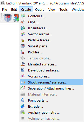
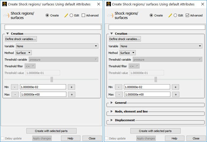
Figure 5.81: Shock Regions/Surfaces Icon

Figure 5.82: Feature Panel - Shock Regions/Surfaces

Create/Edit	Toggles that control whether a new part will be created, or whether you are editing existing part(s). Note: When editing, the changes will be applied to those parts which have the small pencil icon next to them in the Parts list.
Advanced	Will open additional features for more advance control of the Part.
Desc	The name of the part to be created or being edited.
Creation
Variable	A list of variables used to create the shock surface via Surface method. These variables are specified via those SET in the Define Shock Variables list. Note: This list is not used for the Region method. The Region method only uses pressure as the creation variable.
Define Shock Variables...	Opens the Shock Variable Settings dialog which allows the user to identify and set the dependent variables used in computing the shock parts. This dialog has a list of current accessible variables from which to choose. Immediately below is a list of dependent variables with corresponding text field and SET button. The variable name in the list is tied to a dependent variable below by first highlighting the listed variable, and then clicking the corresponding dependent variable's SET button, which inserts the listed variable into its corresponding text field. 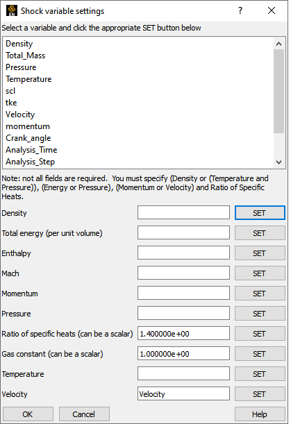Not all text fields are required. Although you must specify either Density or Pressure, Temperature, and Gas Constant; either Energy or Pressure; either Velocity or Momentum; and the Ratio of Specific Heats. A default constant value is supplied for the Ratio of Specific Heats and the Gas Constant which may be changed or specified by a scalar variable name. Clicking OK activates all specified dependent variables and closes the dialog.
Method	Opens a pop-up dialog for the specification of which type of method, to use to compute the vortex cores in the 3D field. These options are: Surface Scheme that uses maximal density or pressure gradients in the streamwise direction to locate candidate shock surfaces. (See Algorithms above). Region Scheme that uses flow physics based on the mach vector coupled with pressure gradient to locate candidate shock regions. (See Algorithms above.)
Threshold Variable	A list of possible variables that you may use to help filter out unwanted areas. This list includes the shock threshold variables `SHK_` which gets created when you Create/Update* a shock part.
Threshold Filter	Relational operators used to filter out shock areas.
	>=	Filter out any areas greater than or equal to the Threshold Value.
	<=	Filter out any areas less than or equal to the Threshold Value (default).
Threshold Slider Bar	Used to change the Threshold Value in increments dependent on the Min and Max settings. The stepper button on the left (and right) of the slide bar is used to decrement (and increment) the Threshold value
	Min	The minimum value of the Threshold Variable. The stepper button on the left (and right) side of the Min text field is used to decrease (and increase) the order of magnitude, or the exponent, of the Min value.
	Max	The maximum value of the Threshold Variable. The stepper button on the left (and right) side of the Max text field is used to decrease (and increase) the order of magnitude, or the exponent, of the Max value.
Threshold Value	The value at which to filter the shock areas.
Create with selected parts	Creates a Shock regions/surfaces part using the selected Part(s) in the Parts list.
Delay update	Checking this box will cause EnSight to not apply any changes made until you hit the Apply Changes button. When not checked, the changes are applied as you make them.
Apply Changes	Applies any changes made. Only active when Delay update is on.

See Feature Panel Turndowns Common To All Part Types for a detailed discussion of the remaining Feature Panel turn-down sections which are the same for all Parts.

Note: Shock Surface feature extraction does not work with multiple cases.

Troubleshooting Shock Surfaces/Regions

Problem	Probable Causes	Solutions
Error creating shock part	Non-3D part selected in part list	Highlight 3D flow field part
No shock part created	Flow field part subsonic	No shock in subsonic regions
No shock part created	Shock dependent variables defined with incorrect units, i.e. since Region method uses density and mach, if file variables are pressure, temperature, and velocity, then density (and therefore mach) is dependent on gas constant. By default this value is 287 (Nm/KgK)	Make sure dependent variables have correct units. i.e. gas constant may need to be 1716 (ft-lb/slugDegR), or some other value rather than the default
No to little shock part created	Threshold value too large for < operation	Decrease threshold value

5.2.15. Subset Parts

EnSight enables you to create and modify Subset Parts from ranges of node and/or element labels of model parts. The Subset Parts feature allows you to isolate contiguous and/or non-contiguous regions of large data sets, and apply the full-range of feature applications and inspection provided by EnSight.

Subset Parts can only be created from parts that have node and/or element labels. Therefore, Subset Parts can not be created from any Created Parts, because the only parts that can have node and element labels are Model Parts such as parts built from file data, Merged Model Parts, or Computational Mesh Model Parts (parts created via the periodic computational symmetry Frame attribute). Model Parts that do not have given or assigned node and/or element labels can not be used to create Subset Parts.

Subset Parts are created and reside on the server. They are Created Parts that provide proper updating of all dependent parts and variables.

Subset Parts are created and modified by specifying parent parts, as well as their node and/or element labels. Node and/or element labels can be displayed and filtered interactively according to global View and local Part attributes.

Clicking once on the Subset parts icon (if you have customized the Feature Ribbon to have it visible) or selecting Subset parts... in the Create menu, opens the Feature Panel for Subset parts. This editor is used to both create and edit Subset parts.

Figure 5.83: Subset Parts Icon

Figure 5.84: Feature Panel - Subset Parts

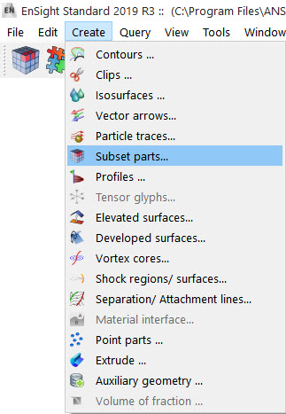
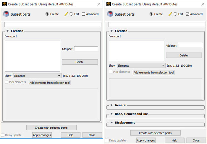
Create/Edit	Toggles that control whether a new part will be created, or whether you are editing existing part(s). Note: When editing, the changes will be applied to those parts which have the small pencil icon next to them in the Parts list.
Advanced	Will open additional features for more advance control of the Part.
Desc	The name of the part to be created or being edited.
Creation
From Part	List reflecting the parent parts that have been added to the list. Selecting a part in this list displays any corresponding element or node range specifications in the Show List.
Show	Opens a pulldown menu for selecting which type of part entity you wish to include (or have included) in your Subset Part. The Show options are:
	Elements	show any specified element label ranges
	Nodes	show any specified node label ranges
Add part	This field specifies the graphical user interface part number you wish to add to the From Part list.
Delete	This button removes any selected entries in the From Part list along with any corresponding element or node range specifications in the Show List.
Show List	This field specifies the label ranges of Elements and/or Nodes wanted for the Subset Part that correspond to the selected part in the From Part list. The Elements or Nodes are specified as a range as the example indicates, i.e. (Ex. 1,3,8,9,100-250).
Pick elements	This toggle enables element picking from the graphics window. Elements will be picked using the pick selection which by default is the P key.
Add Elements from Selection Tool	Activate the selection tool, and adjust your selection window then click this button to select all the elements within the window.
Create with selected parts	Creates a Profile part using the selected Part(s) in the Parts list.
Delay update	Checking this box will cause EnSight to not apply any changes made until you hit the Apply Changes button. When not checked, the changes are applied as you make them.
Apply Changes	Applies any changes made. Only active when Delay update is on.

See Feature Panel Turndowns Common To All Part Types for a detailed discussion of the remaining Feature Panel turn-down sections which are the same for all Parts.

5.2.16. Tensor Glyph Parts

Tensor glyphs visualize the direction and tension/compression of the eigenvectors at discrete points (at nodes or at element centers) for a given tensor variable.

Tensor glyph Parts are dependent Parts known only to the client. They cannot be used as a parent Part for other Part types and cannot be used in queries. As dependent Parts, they are updated anytime the parent Part and/or the creation tensor variable changes (unless the general attribute Active flag is off).

Tensor glyphs can be filtered to show just the tensile or compressive eigenvectors. Further, the visibility for each of the eigenvectors (Major, Middle, and Minor) can be controlled.

Tensor glyphs will appear for each of the nodes/elements for the Parent part's visual Representation. Therefore, for a border Representation of a Part, only the border nodes/elements will be candidates for a tensor glyph.

The tensile and compressive eigenvectors can be visualized by modifying the tensile/compressive component's line width and color.

Clicking once on the Tensor glyphs icon (if you have customized the Feature Toolbar to have it visible) or selecting Tensor glyphs... in the Create menu, opens the Feature Panel for Tensor glyph parts. This editor is used to both create and edit Tensor glyph parts.

Figure 5.85: Tensor Glyph Icon

Figure 5.86: Feature Panel - Tensor Glyph

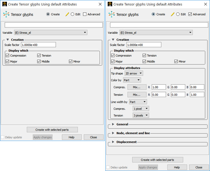
Create/Edit	Toggles that control whether a new part will be created, or whether you are editing existing part(s). Note: When editing, the changes will be applied to those parts which have the small pencil icon next to them in the Parts list.
Advanced	Will open additional features for more advance control of the Part.
Desc	The name of the part to be created or being edited.
Variable	The tensor variable used for the glyphs.
Creation
Scale Factor	The size of the tensor glyph.
Display Which	Controls which eigenvectors will be displayed.
	Compression	Show the eigenvectors that are in compression
	Tension	Show the eigenvectors that are in tension
	Major	Show the major eigenvector
	Middle	Show the middle eigenvector
	Minor	Show the minor eigenvector
Display Attributes
Tip Shape	Opens a pop-up menu to select the tip shape.
	None	Displays eigenvectors as lines with no tips.
	Normal	Displays classical tips.
	Triangles	Displays triangle tips.
Tip Size	Controls the size of the tips.
Color By	The tensor glyphs can be colored according to the part color, or have a separate color for compression and tension.
	Compression Color	Specify the compressive color
	Tension Color	Specify the tensile color
Line Width By	The tensor glyphs can use the part line width, or have a separate line width for compression and tension.
	Compression Line Width	Specify the compressive line width
	Tension Line Width	Specify the tensile line width
Create with selected parts	Creates a Profile part using the selected Part(s) in the Parts list.
Delay update	Checking this box will cause EnSight to not apply any changes made until you hit the Apply Changes button. When not checked, the changes are applied as you make them.
Apply Changes	Applies any changes made. Only active when Delay update is on.

See Feature Panel Turndowns Common To All Part Types for a detailed discussion of the remaining Feature Panel turn-down sections which are the same for all Parts.

(see Parts Quick Action Icons and Create Tensor Glyphs).

Troubleshooting Tensor Glyphs

Problem	Probable Causes	Solutions
No tensor glyphs created	No real eigenvectors exist.	None
	Scale Factor too small.	Increase Scale Factor.
	Parent parts have non-visual attributes.	Re-specify parent parts or modify parent part's Element Representation.
	Parent parts do not contain selected tensor variable.	Re-specify parent parts.
Too many glyphs	Parent parts have too many points at which tensor glyphs are to be displayed.	Consider using a grid clip as the parent part.

5.2.17. Vector Arrow Parts

Vector Arrows visualize the magnitude and direction of a vector variable at discrete points (at nodes, element vertices, or at the center of elements).

Other features can visualize magnitude, but Vector Arrows also show direction.

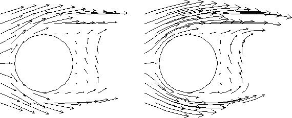
Vector arrow Parts are dependent Parts known only to the client. They cannot be used as a parent Part for other Part types and cannot be used in queries. As dependent Parts, they are updated anytime the parent Part and/or the creation vector variable changes (unless the general attribute Active flag is off).

Vector arrows can be filtered according to low and/or high threshold values.

Vector arrows can emanate from the available nodes of the parent Part(s), the available element vertex nodes of the parent Part(s), or the available element centers of the parent Part(s) which pass through the filter successfully. The nodes and elements available in the parent Part are based on the visual Representation of the Part. Therefore, for a border Representation of a Part, only the border elements and associated nodes are candidates.

Vector arrows can have straight shafts representing the vector at the originating location, or be the segment of a streamline emanating from the originating location (curved). Straight vector arrows are displayed relatively quickly, while curved vector arrows can be time consuming.

Different tip styles, sizes, and colors can be used to enhance vector arrow display.

To quickly create vector parts, right-click in the graphics window on a surface and drag down to vector arrows, and vector arrows will automatically appear (if there's only one vector variable) or you will be prompted for which vector variable to use to create vector variables and they will automatically appear. Left click the arrows and when a green, cross-shaped handle (click and go handle) appears, drag it left and right to scale the arrows.

Clicking once on the Vector arrows icon (which is in the Feature Ribbon by default) or selecting Vector arrows... in the Create menu, opens the Feature Panel for Vector arrow parts. This editor is used to both create and edit Vector arrow parts.

Figure 5.87: Vector Arrow Icon

Figure 5.88: Feature Panel - Vector Arrows

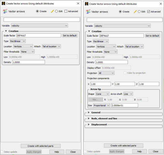
Create/Edit	Toggles that control whether a new part will be created, or whether you are editing existing part(s). Note: When editing, the changes will be applied to those parts which have the small pencil icon next to them in the Parts list.
Advanced	Will open additional features for more advance control of the Part.
Desc	The name of the part to be created or being edited.
Variable	Choose the variable to use for creating the vector arrow part from the pulldown.
Creation
Scale Factor / Time	When Type is Rectilinear, this field specifies a scale factor to apply to the vector values before displaying them. Scaling is usually necessary to control the visual length of the vector arrows since the vector values may not relate well to the geometric dimensions. Can be negative, causing the vector arrows to reverse direction. When Type is Rect. Fixed, this field specifies the length of the arrows in units of the model coordinate system. Can be negative, causing the vector arrows to reverse direction. When Type is Curved, this field specifies the duration time for streamlines forming the shaft of curved vector arrows. Is an indication of the length of the curved vector arrow.
Set to Default	Sets Scale Factor value to a computed reasonable value based on the vector variable values and the geometry.
Type	Opens a pop-up menu for selection of shaft-type of vector arrows. Options are: Rectilinear arrows have straight shafts. The arrow points in the direction of the vector at the originating location. The length of the arrow shaft is determined by multiplying the vector magnitude by the scale factor. Rect. Fixed arrows have straight shafts. The arrow points in the direction of the vector at the originating location. The length of the arrow shaft is determined by the scale factor. It is independent of the vector variable. Curved arrows have curved shafts. The arrow is actually a streamline emanating from the originating location. It represents the path that a massless Particle would follow if the flow field was steady state. For this option, the Scale Factor changes to Time. Time is the amount of time the streamline is allowed to take and is an indication of how long the arrow will be. Tip: Since curved arrows can take a significant amount of time (depending on the number of originating locations), the setting of a proper Time value is critical. The best way to do this is to first do a single Particle trace at a representative location with the estimated Time value as the Max Time. A quick iteration or two on the value here could save considerable time for the curved vector arrow computation.
Location	Opens a pop-up dialog for the selection of root-location of arrow shafts. The options are:
	Node	arrows originate from each node of the parent Part(s). Note: Discrete Particles Parts must use Node option.
	Vertices	arrows originate only from those nodes at the vertices of each element of the parent Part(s) (that is, arrows are not displayed at free nodes or mid-side nodes).
	Element Center	arrows originate from the geometric center of each element of the parent Part(s).
Attach	Specifies if the tip or tail should be located at the Location specified. This option is not available for Type → Curved.
	Tail at location	The tail of the vector arrow is located at the Location specified.
	Tip at location	The tip of the vector arrow is located at the Location specified.
Filter Thresholds	Selection of pattern for filtering Vector Arrows according to magnitude. Options are: None displays all the vector arrows. No filtering done. Low displays only those arrows with magnitude above that specified in the Low field. Filters low values out. Band displays only those arrows with magnitude below that specified in the Low field and above that specified in the High field. Filters the band out. High displays only those arrows with magnitude below that specified in the High field. Filters the high values out Low_High displays only those arrows with magnitude between that specified in the Low field and that specified in the High field. Filters out low and high values.
Density	The fraction of the parent's nodes/elements which will show a vector arrow. A value of 1.0 will result in a vector arrow at each node/element, while a value of 0.0 will result in no arrows. If between these two values, the arrows will be distributed randomly at the specified density. There is no check for duplicates in the random distribution of arrows. It is entirely possible that when you specify a density of 0.25 in a model containing 100 nodes you only get 15 unique locations with 10 duplicates. It will appear that only 15 arrows show up, but there are actually 25 with 10 duplicates.
Display offset	This field specifies the normal distance away from a surface to display the vector arrows. A positive value moves the vector arrows away from the surface in the direction of the surface normal. Note: There is a hardware offset that will apply to contours, vector arrows, separation/attachment lines, and surface restricted particle traces that can be turned on or off in the View portion of Edit → Preferences. This preference (Use graphics hardware to offset line objects...) is on by default and generally gives good images for everything except move/draw printing. This hardware offset differs from the display offset in that it is in the direction perpendicular to the computer screen monitor (Z-buffer). Therefore, for viewing, you may generally leave the display offset at zero. But for printing, a non-zero value may become necessary so the arrows print cleanly.
Projection	Opens a pop-up menu to allow selection of which vector components to include when calculating both the direction and magnitude of the vector arrows. The vector components at the originating point are always first multiplied by the Projection Components (see below). Then one of the following options is applied:
	All	to display a vector arrow composed of the Projection-Component-modified X, Y, and Z components.
	Normal	to display a vector which is the projection of the All vector in the direction of the normal at the originating location.
	Tangential	to display a vector which is the projection of the All vector into the tangential plane at the originating location.
	Component	to display both the Normal and the Tangential vectors.
	The All, Normal, and Tangential options produce a single vector per location, while the Component option produces two vectors per location. If selection is not applicable to a Particular element, that element's vector arrow uses the All projection.
Color by Projection	If the projection is Tangential or Normal and the vector arrow is colored by the vector, then the vector arrow is colored by the Tangential or Normal, respectively.
Projection Components X Y Z	These fields specify a scaling factor for each coordinate component of each vector arrow used in calculating both the magnitude and direction of the vector arrow. Specify 1 to use the full value of a component. Specify 0 to ignore the corresponding vector component (and therefore confine all the vector arrows to planes perpendicular to that axis). Values between 0 and 1 diminish the contribution of the corresponding component, while values greater than 1 exaggerate them. Negative values reverse the direction of the component. Always applied before the Projection options above.
Arrow Tip
Shape	Opens a pop-up menu to select tip shape.
	None	option displays arrows as lines without tips.
	Cone	arrows have a tip composed of a 3D cone. Good for both 2D and 3D fields
	Normal	arrows have two short line tips, similar to the way many people draw arrows by hand. The tip will lie in the X-Y, X-Z, or Y-Z plane depending on the relative magnitudes of the X, Y, and Z components of each individual vector. Suggested for 2D problems.
	Triangles	arrows have a tip composed of two intersecting triangles in the two dominant planes. Good for both 2D and 3D fields.
	Tipped	arrows display the tip of the arrow in any user specified color. Good for both 2D and 3D fields. The color may be specified in the RGB fields or chosen from the Color Selector dialog which is opened by pressing the Mix... button
Arrow Shaft	Opens a pull-down menu to select the arrow shaft type. This option is only available if the arrow tip shape has been set to Cone.
	Line	Draw the arrow shafts as lines
	Solid	Draw the arrow shafts as cylinders which will be shaded according to lighting attributes
Size	Lets you control a scale factor for tip size
	Fixed	sized arrows have tips for which the length is specified in the data entry field to the right of the pop-up menu button. Units are in the model coordinate system
	Proportional	sized arrow tips change proportionally to the change in the magnitude of the vector arrows.
Create with selected parts	Creates a vector arrow part using the selected Part(s) in the Parts list.
Delay update	Checking this box will cause EnSight to not apply any changes made until you hit the Apply Changes button. When not checked, the changes are applied as you make them.
Apply Changes	Applies any changes made. Only active when Delay update is on.

See Feature Panel Turndowns Common To All Part Types for a detailed discussion of the remaining Feature Panel turn-down sections which are the same for all Parts.

See Create Vector Arrows.

Troubleshooting Vector Arrows

Problem	Probable Causes	Solutions
Vector arrows do not match up with their originating locations on one or more of the parent Parts.	Displacements are on for some of the parent Parts, but not others or the parent Parts have been assigned to different coordinate frames	Create separate vector arrow Parts for the parents that will be displaced (or assigned to different frame) and the ones that will not be displaced (or assigned to different frames).
You are displaying several different vector arrow Parts at once and can't tell which is which.	Just too much similar information in the same area.	Use different attributes for the different vector arrow Parts, or better yet, display the conflicting vector arrow Parts on separate Part copies which have been moved apart.
You are trying to display vector arrows on a Discrete Particle Part, but can't get them to show up	Arrow Location set to Vertices (the default).	Set the Arrow Location to Nodes.
	No vector data provided for the Discrete Particle dataset, therefore values all set to zero when read into EnSight.	Provide vector data for the particles. Specify in the Measured results file. See Variables List Panel.
Vector arrows do not print well	See Display Offset discussion above.	Enter a non-zero Display Offset.

5.2.18. Vortex Core Parts

Vortex cores help visualize the centers of swirling flow in a flow field. EnSight creates vortex core segments from the velocity gradient tensor of 3D flow field part(s). Core segments can then be used as emitters for ribbon traces to help visualize the strength and nature of the vortices.

5.2.18.1. Velocity Gradient Tensor

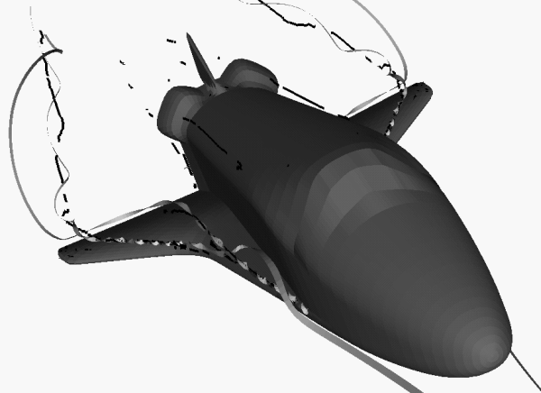
EnSight automatically pre-computes the velocity gradient tensor for all 3D model parts prior to creating the vortex cores. Since this variable is automatically created, all subsequent 3D model parts created will also have this tensor computed.

Note: The velocity gradient tensor variable will continue to be created and updated for all 3D model parts until it is deactivated.

This tensor variable behaves like any other created tensor variable, and may be deactivated in the Variables List.

5.2.18.2. Thresholding

Core segments may be filtered out according to the settings of a threshold variable, value, and relational operator. Most active variables can be used as threshold variables. Thresholding was implemented to help the user filter-out, or view portions of the core segments according to variable values.

When vortex core parts are Created/Updated, the vorticity magnitude scalar variable fx_vortcore_streng is created to help you threshold unwanted core segments according to these scalar values. (This is the magnitude (RMS) of the vorticity as defined in Main Menu)

Due to the difference in algorithms, some segments produced may not be vortex cores (see Caveats). Therefore, the need for a filtering mechanism that filters out segments according to different variables arose and has been provided via thresholding options.

5.2.18.3. Algorithms

Currently, vortex cores are calculated according to two algorithms based on techniques outlined by Sujudi, Haimes, and Kenwright (see References below). Both techniques are linear and nodal. That is, they are based on decomposing finite elements into tetrahedrons and then solving closed-form equations to determine the velocity gradient tensor values at the nodes. Also, any variable with values at element centers are first averaged to element nodes before processing.

The eigen-analysis algorithm uses classification of eigen-values and vectors to determine whether the vortex core intersects any faces of the decomposed tetrahedron. The vorticity based algorithm utilizes the fact of alignment of the vorticity and velocity vectors to determine core intersection points.

5.2.18.4. References

Please refer to the following references for more detailed explanations of pertinent concepts and algorithms.

D. Banks, B. Singer, "Vortex Tubes in Turbulent Flows: Identification, Representation, Reconstruction", IEEE Visualization '94, 1994

D. Sujudi, R. Haimes, "Identification of Swirling Flow in 3-D Vector Fields",AIAA-95-1715, Jun. 1995

D. Kenwright, R. Haimes, "Vortex Identification - Applications in Aerodynamics",IEEE Visualization '97, 1997

M. Roth, R. Peikert, "A Higher-Order Method For Finding Vortex Core Lines",IEEE Visualization '98, 1998

R. Haimes and D. Kenwright, On the Velocity Gradient Tensor and Fluid Feature Extraction", AIAA-99-88, Jan. 1999

R. Peikert, M. Roth, "The 'Parallel Vectors' Operator - a vector field visualization primitive", IEEE Visualization '99, 1999

D. Kenwright, T. Sandstrom, GEL, NASA Ames Research Center, 1999

R. Haimes, D. Kenwright, The Fluid Extraction Toll Kit,Massachusetts Institute of Technology, 2000

R. Haimes, K. Jordan, "A Tractable Approach to Understanding the Results from Large-Scale 3D Transient Simulations", AIAA-2000-0918, Jan. 2001

5.2.18.5. Caveats

Due to the linear implementation of both the eigen-analysis and vorticity algorithms, they both have problems finding cores of curved vortices. In addition, testing has shown that both algorithms usually fail to predict vortex core segments in regions of weak vortices.

Note: For regions of weak vortices consider using the Lambda2 or Q-criteria calculator functions. See Variable Creation.

Since the eigen-analysis method finds patterns of swirling flow, it can also locate swirling flow features that are not vortices (especially in the formation of boundary layers). These non-vortex core type segments can sometimes be filtered out via thresholding (see Thresholding ). In addition, the eigen-analysis algorithm may produce incorrect results when the flow is under more than one vortex, and has a tendency to produce core locations displaced from the actual vortex core.

The vorticity based method does not seem to exhibit the problem of producing core segments due to boundary layer formations, because the stress components of the velocity gradient tensor have been removed in the formation of the vorticity vector. Therefore, the vorticity method seems to produce longer and more contiguous cores - in most cases; and therefore, the reason for including both algorithms.

5.2.18.6. Access

Clicking once on the Vortex cores icon (if you have customized the Feature Ribbon to have it visible) or selecting Vortex cores... in the Create menu, opens the Feature Panel for Vortex core parts. This editor is used to both create and edit Vortex core parts.

Figure 5.89: Vortex Core Icon

Figure 5.90: Feature Panel - Vortex Cores

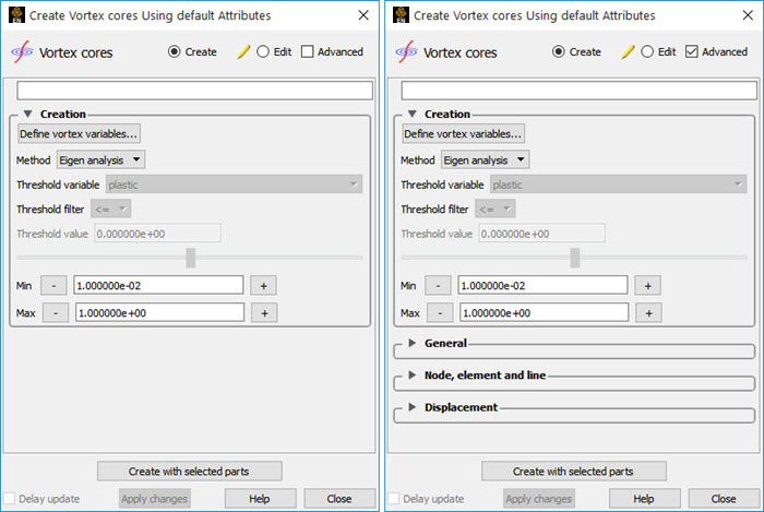
Create/Edit	Toggles that control whether a new part will be created, or whether you are editing existing part(s). Note: When editing, the changes will be applied to those parts which have the small pencil icon next to them in the Parts list.
Advanced	Will open additional features for more advance control of the Part.
Desc	The name of the part to be created or being edited.
Creation
Define Vortex Variables...	Opens the Vortex Core Variable Settings dialog which allows the user to identify and set the dependent variables used in computing the vortex cores. This dialog has a list of current accessible variables from which to choose. Immediately below is a list of dependent variables with corresponding text field and SET button. The variable name in the list is tied to a dependent variable below by first highlighting a listed variable, and then clicking the corresponding dependent variable’s SET button, which inserts the listed variable into its corresponding text field. 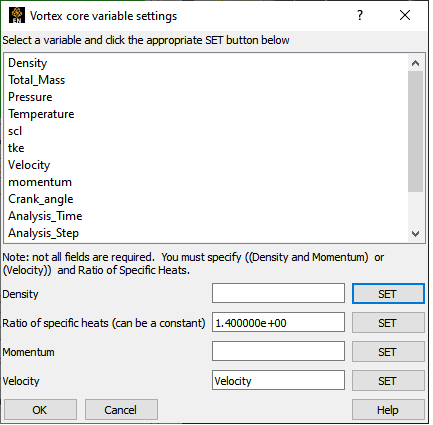All text fields are required, except you may specify either Density and Momentum (which permits velocity to be computed on the fly), or just Velocity. A default constant value is supplied for the Ratio of Specific Heats which may be changed or specified by a scalar variable name. Clicking OK activates all specified dependent variables and closes the dialog.
Method	Opens a pop-up dialog for the specification of which type of method to use to compute the vortex cores in the 3D field. These options are: Eigen Analysis Scheme that uses eigen-analysis on the Velocity gradient tensor to compute the vortex core segments. (See Algorithms above). Vorticity Scheme that uses the vorticity vector from the anti-symmetric portions of the velocity gradient tensor to compute the vortex core segments. (See Algorithms above).
Threshold Variable	A list of possible variables that you may use to help filter out vortex core segments. This list includes the vorticity magnitude scalar variable (named `fx_vortcore_streng`) which gets created when you Create/Update a vortex core part.
Threshold Filter	Relational operators used to filter out line segments.
	>=	Filter out any core segments greater than or equal to the Threshold Value.
	<=	Filter out any core segments less than or equal to the Threshold Value (default).
Threshold Value	The value at which to filter the vortex core segments.
Threshold Slider Bar	Used to change the Threshold Value in increments dependent on the Min and Max settings. The stepper button on the left (and right) of the slide bar is used to decrement (and increment) the Threshold value
	Min	The minimum value of the Threshold Variable. The stepper button on the left (and right) side of the Min text field is used to decrease (and increase) the order of magnitude, or the exponent, of the min value.
	Max	The maximum value of the Threshold Variable. The stepper button on the left (and right) side of the Max text field is used to decrease (and increase) the order of magnitude, or the exponent, of the Max value.
Create with selected parts	Creates a Separation and Attachments part using the selected Part(s) in the Parts list.
Delay update	Checking this box will cause EnSight to not apply any changes made until you hit the Apply Changes button. When not checked, the changes are applied as you make them.
Apply Changes	Applies any changes made. Only active when Delay update is on.

See Feature Panel Turndowns Common To All Part Types for a detailed discussion of the remaining Feature Panel turn-down sections which are the same for all Parts.

Note: Once a Vortex Core feature extraction calculation has been completed, it is no longer possible to replace nor add case(s). However, if multiple cases have already been loaded, then it is possible to use the Vortex Core feature extraction on each of the cases.

Troubleshooting Vortex Cores

Problem	Probable Causes	Solutions
Error creating vortex cores	Non-3D part selected in part list	Highlight 3D part
Undefined (colored by part color) regions on vortex cores	Vortex core line segment node was not mapped within a corresponding 3D field element	Make sure corresponding 3D field part is defined.

5.2.19. Auxiliary Geometry

Auxiliary Geometry helps frame parts for visual effects. These geometries can be texture-mapped for environmental reference, as well as display cast part shadows when combined with directional lighting and ray-traced images.

5.2.19.1. Access

Clicking once on the Auxiliary Geometry icon (if you have customized the Feature Ribbon to have it visible) or selecting Auxiliary Geometry... in the Create menu, opens the Feature Panel for Auxiliary Geometry parts. This editor is used to both create and edit Auxiliary Geometry parts.

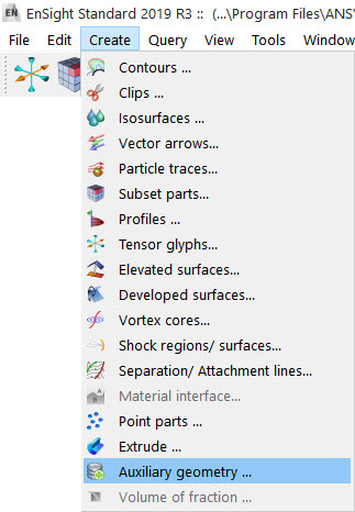
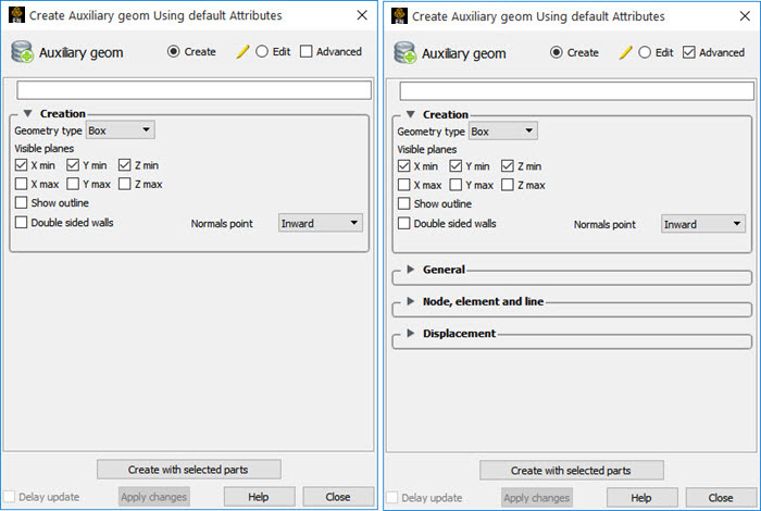
Figure 5.91: Auxiliary Geometry Icon

Figure 5.92: Feature Panel - Auxiliary Geometry

Create/Edit	Toggles that control whether a new part will be created, or whether you are editing existing part(s). Note: When editing, the changes will be applied to those parts which have the small pencil icon next to them in the Parts list.
Advanced	Will open additional features for more advance control of the Part.
Desc [text field]	The name of the part to be created or being edited.
Creation
Geometry Type	To specify which type of geometry to be created/edited. The options are:
	Box	A box whose dimensions are the bounding box of the selected part(s) with visible sides, top & bottom planes. Currently Box is the only option, but it is a pulldown because more may be added in the future.
	Visible planes	Controls which planes (sides of the box) that will be created. X min Show the x-min plane Y min Show the y-min plane Z min Show the z-min plane X max Show the x-max plane Y max Show the y-max plane X max Show the z-max plane
	Show outline	Show the outline of the specified geometry type.
	Double sided walls	Create two walls with opposing normals (an inside and an outside surface for each wall). This is to overcome raytracing error tolerance limitations. Double sided walls might be useful, for example, to better compute the shadow effect on the edge or corner of the box. If a single wall is used, the edge can be mistakenly bright or dark. With an extra layer, the lighting is correct.
	Normals point	A pulldown menu for the specification of which direction to create surface normals off the walls. Options are inward or outward. This is usually not important for OpenGL rendering, and is primarily for raytracing. If double sided walls is ON, then this option is ignored. Inward (default) Normals off the wall point into the part. Outward Normals off the wall point out from the part. For a single layered box (Double sided walls off), the boundary planes are created by default with normals pointing inward. For most scenes where the auxiliary geometry is designed to provide a backdrop to the model, an inward normal is the right choice for raytracing. And outward normal is provided for rare situations where the auxiliary geometry is not just a backdrop and you are using less common backdrop geometry, for example, a glass material, which needs to know the entry point and exit point correctly. Flipping the normal direction may provide a better raytrace rendering in this rare situation.
Create with selected parts	Creates an Auxiliary geometry part using the selected Part(s) in the Parts list. Note: You can still click on a wall and drag it to a different location.

See Feature Panel Turndowns Common To All Part Types for a detailed discussion of the remaining Feature Panel turn-down sections which are the same for all Parts.

Troubleshooting Auxiliary Geometry

Problem	Probable Causes	Solutions
Error creating auxiliary geometry	No parts selected in part list	Must select existing part(s) in the Parts list prior to creating auxiliary geometry that will bound the part(s).

5.2.20. Filter Parts

A Filter part is a collection of elements and nodes from a list of parent parts that pass up to 6 different filters. The filters specify what will be filtered out. For example, if the filter was set up for Pressure > .5 the filter part will contain all the nodes/elements where the Pressure <= .5.

Up to 6 filters can be applied. They are assumed to all be of an AND logical operator. The algorithm will filter out all nodes that are not in use by elements, for example, nodes in the filter part are only those used for element connectivity.

This part type will not generate geometry/variables for parts not defined on the EnSight server such as contours, profiles, particle traces, vector arrows and tensor glyphs.

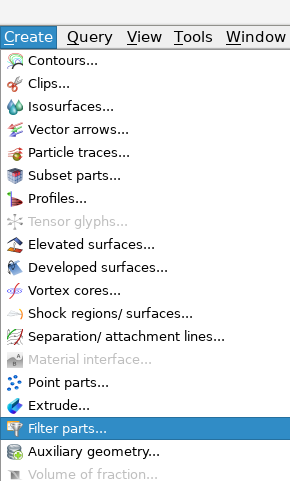
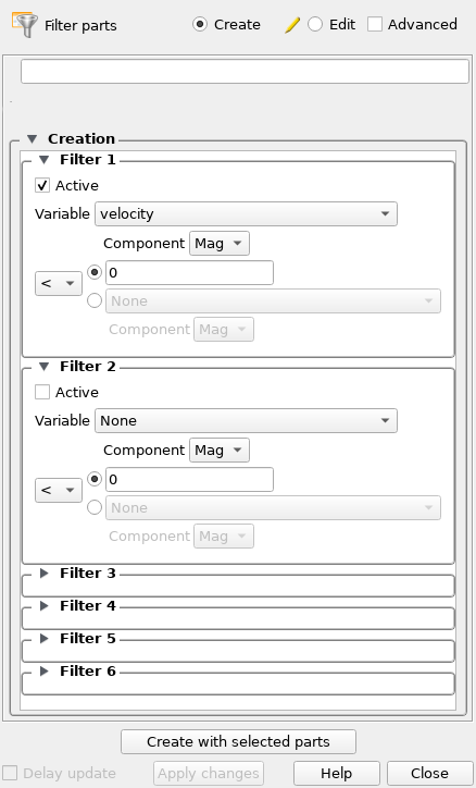
Create/Edit	Toggles that control whether a new part will be created, or whether you are editing existing part(s). Note: When editing, the changes will be applied to those parts which have the small pencil icon next to them in the Parts list.
Advanced	Will open additional features for more advance control of the Part.
Desc	The name of the part to be created or being edited.
Active	Toggle on to make the defined filter active.
	Variable	A scalar or vector variable or a coordinate axis to filter.
	Component	if Variable is a vector then choose Magnitude, X, Y, or Z components
	Test	One of <, > = or != for the filter test. The test can either be against a constant value or be against another scalar, vector or coordinate component. If the test is against a vector variable you can specify if you want to vector magnitude or a component.
Create with selected parts	Creates an Auxiliary geometry part using the selected Part(s) in the Parts list. Note: You can still click on a wall and drag it to a different location.
Delay update	Checking this box will cause EnSight to not apply any changes made until you hit the Apply Changes button. When not checked, the changes are applied as you make them.
Apply Changes	Applies any changes made. Only active when Delay update is on.

See Create Filter Parts in the Ansys EnSight How-To Manual.