


The following topics are included in this section:
EnSight has an architecture designed for compatibility with a variety of compute environments - ranging from desktops to distributed memory clusters perhaps located at remote locations. The extent to which you utilize or ignore this architecture is up to you.
As an overview, EnSight always has, at minimum, two processes running. The process that you interact with on your desktop is called the client. It is responsible for user interaction as well as all graphics functions. The other process that is running when you launch EnSight is the server. The server process reads the data and extracts the portion (geometry, variables, queries, etc.) that you wish to view - either as 3D geometry or queries of various kinds. The server process can run on the same machine as the client but may also run on other systems - in which case the two processes communicate with each other across the network.
For the most part, users will find satisfactory performance with EnSight transparently running client and server processes on their same machine. However, EnSight has much more powerful options.
Moving your large dataset from a compute server to your desktop for visualization is a waste of time and resources. You should never need to move large datasets! The EnSight server should always run on the compute system(s) that generated the large data. As your datasets become larger, the EnSight client can run on your local machine with a good graphics hardware card and the EnSight server can be run on your big memory solver machine near the data.
EnSight sometimes uses multiple servers. It uses multiple servers to read multiple datasets, or multiple servers to partition a single, large dataset or to cache transient data for faster time change. For example, the client can compare multiple datasets by connecting to multiple servers; each separate server loads its own dataset (called a case). Or, a single, large dataset can be spatially partitioned among a number of servers with a server of server (SOS) acting as a communication hub between the servers and the client. And finally a single, large, transient dataset can be automatically temporally partitioned among multiple servers (each with one full timestep) to speed up the time change using caching.
Data on the server is inherently 3D. With one exception (volume rendering), data on the client is inherently 2D polygons, that is, 3D information has been reduced one dimension by the time you see it on the client.
EnSight can use multiple clients. For extremely large datasets that result in an extremely large number of 2D polygons on the client, multiple clients can be used to overcome rendering problems. EnSight can subdivide the rendering problem into manageable portions using multiple clients.
EnSight writes temporary files for caching purposes, to the directory defined by the environmental variable CEI_TMPDIR (if set) or TMPDIR. These files will be prefixed Ensi + pid_ where pid is the process id using 6 digits, that is if pid=325 and the generated temporary file extension is 12, then you have Ensi000325_12. Temporary files are written during isosurface creation, command file recording, certain licensing operations and certain backup operations.
Each time you read a new set of data you open a case. Cases can be deleted, added, or replaced. You can have multiple cases loaded simultaneously and each case can be a different format and can contain different geometric and variable information.
A case can be transient - meaning something (geometry and/or variables) is changing over time - or static meaning steady state with no data changing over time.
Each case will contain parts and possibly (usually) variables.
Loading multiple cases is usually used to perform comparisons between similar solver runs or to composite solutions from an assembly.
A case is read via a Data Reader. Multiple data readers and translators currently exist and are constantly being worked on and expanded. They consist of the following 4 types:
Type 1 - Included Readers - Are accessed by choosing the desired format in the Data Reader dialog. These include common data formats as well as a number of readers for commercial software.
Type 2 - Not Included User-Defined readers - A number of User-Defined Readers have been authored by EnSight users, but are not provided with EnSight. They are often available via a third party.
Type 3 - Stand - Alone Translators - May be written by the user to convert data into EnSight format files. A complete description of EnSight formats may be found in EnSight Data Formats of this manual. Several translators are provided with EnSight. Others may be available from third parties.
Type 4 - EnSight Format - A growing number of software suppliers support the EnSight format directly, that is an option is provided in their products to output data in the EnSight format.
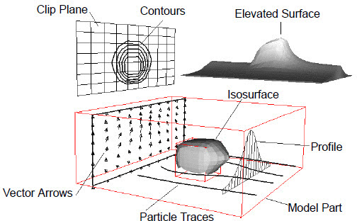
The Part is the fundamental visualization entity in EnSight. Virtually every post-processing task you perform will involve a Part, therefore it is vital to understand how parts work.
A part is a collection of nodes and elements that are grouped together and share the same attributes. When you start EnSight, you either read directly or interactively extract parts from the data files. Parts which come from the original dataset are referred to as model parts. Other parts created within EnSight, are referred to as created (or dependent) parts. Model Parts are defined by the data readers and are usually a logical grouping of nodes and elements as defined by the solver. It might be a material or property or perhaps a defined geometric entity such as a wheel or inlet.
| Definition |
EnSight uses a computational grid and has no concept of parametric surfaces/volumes. |
| Computational Grid |
The computational grid (or mesh) used by EnSight is either an unstructured definition (where each mesh element is defined) or a structured definition (an IJK definition) defining a rectilinear or curvilinear space. It is also possible to have a mixed definition where some parts are unstructured and other parts are structured. |
| Nodes (Vertices) |
Nodes - or sometimes referred to as vertices - are a 3d definition given by a x, y, z coordinate in reference to the model coordinate space. |
| Elements |
Are shapes defined by connecting Nodes. EnSight supports linear and quadratic elements as well as n-sided and n-faced elements. There are 0D, 1D, 2D, and 3D elements. See Preference and Setup File Formats for a definition of the various elements supported by EnSight. |
Structured data does not directly define the elements in use but rather implies quads (in 2D) or hexahedra (3D) elements. These elements may also be modified by Iblanking which may result in the corners of the elements collapsing to form new element types.
When you read data you will choose the file name that will be read and set the format and options for the file. Then you will choose one of two options, either to load all the parts or to select parts to load.

The option will read the specified data (the case) and create, that is load, all of the parts into EnSight. The other option - - will read the data but will not load any parts. This second option will allow you to select on a per part basis which parts will be loaded into EnSight. This load process is performed through the Part List.
The Part List contains all parts that have been read in (loaded) from your specified data file as well as those created within EnSight. Additionally, it may show model parts from the data that are not already loaded. These are referred to as Loadable Parts or LPARTs.
LPARTs may be loaded zero or more times. You may choose not to load a particular part from a data set if it is not needed for the visualization or analysis of the case. This is advantageous to save memory and processing time. You may also choose to load a part multiple times - so you could, for example, color the part by multiple variables at the same time in multiple viewports.
LPARTs are shown as grayed out parts in the Part List. You can load a LPART by selecting the part(s) and performing a right-click operation to Load part.
Attributes define how a part appears and how it is created (in case of created parts). All loaded parts have attributes.
The attributes that control how a part appears are referred to as general or visual attributes. All part types have these same general attributes and include settings such as visibility, line width, color, lighting parameters, etc.
Created parts have creation attributes, settings which specify how the part is created. Each part type will have a different set of creation attributes.
Element Representation
One of the general attributes that deserves some discussion in this overview is Element Representation.
At the start of this chapter the EnSight architecture was briefly discussed, indicating that the server has the data from the case you have loaded and the client shows the extracts of data that you desire. The less data you extract to the client the smaller the memory requirements and higher the performance. One way to minimize the data sent to the client for visualization is to take advantage of the Element Representation attribute.
Element Representation has no effect whatsoever on the data stored and used on the EnSight server process. It only effects what is sent to the client for display. Except for the volume representation, no 3D elements are ever sent to the client. Even when a 3D element is viewed (Full representation) it is viewed on the client as a set of 2D faces for the 3D element.
The choices for Element Representation are:
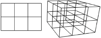
| Full |
The client receives all of the vertices, as well as the definition for all 0D, 1D, and 2D elements and all of the element faces for 3D elements. It is usually a mistake to load parts containing 3D element in this mode. 2D parts are usually best loaded in this mode. The image below shows two parts. The part on the left is composed of quad, that is 2D elements, while the part on the right is composed of hexahedra, that is 3D elements. The 3D part is showing all of the faces of all of the 3D elements resulting in clutter in the interior of the part.
|
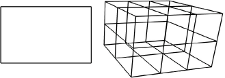
| Border |
The shared edges between 2D elements and the shared faces between 3D elements are removed. Using the same geometry from above, the figure below shows the result of this mode. Note: The 3D part no longer contains interior lines. Border mode is usually the best mode to use for loading 3D parts, and not usually used for 2D parts.
|
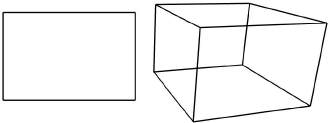
| Feature angle |
This representation works on 2D elements, therefore for 3D parts the server first computes the Border representation. Then given 2D elements, the edge between two elements is removed if the normal between the two elements sharing the edge is less than an angle (default 10 degrees) specified by the user. The result is 1D information on the client that represents sharp edges of the part. The figure below shows the result of feature angle mode. Since the 2D part is planar all of the interior edges are removed. Similarly for the 3D part - since all the exterior bounds of the part are planar - all of the interior edges of each face are removed, leaving just the sharp edges of the box.
|
| Nonvisual |
No data is sent to the client. Note: This is entirely different than loading the part with some other Element Representation and then turning off the visible attribute. The visible attribute simple turns off the rendering of a part. The data has still been sent to the client! This is the recommended mode for parts that do not need to be viewed but will be used for extracting information such as a fluid field around a geometry. |
| Bounding box |
Send only the bounding box geometry to the client for display. |
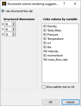
| Volume |
Volume rendering displays all 3D elements at once, drawing each element semi-transparently according to the value of a variable using user-selected x, y, and z dimensions to control the number of elements passed up to the client. This structured, volume rendering uses up to 4 bytes/cell + 72 bytes per pixel on the client graphics card. So a 21x21x21 structured grid with 1kx1k pixel screen, is roughly 40KB + 72 MB, or roughly 72MB.
|
The default Element Representation used by EnSight, unless the data reader for the format you have specified indicates otherwise, is 3D border, 2D full. Meaning 2D elements will be sent to the client in Full mode and 3D elements will be sent in Border mode.
Parts that are created within EnSight are referred to as created (or dependent) parts. The types of parts that you create depend on what features within EnSight you choose to utilize. Any created part is derived from parts that already exist, which is why created parts are sometimes called dependent parts - they depend on the parts from which they were created. The parts that are used to create a dependent part are referred to as parent parts. Any time that a parent part changes, its dependent parts also change. A parent part will change when you change its attributes, or modify the current time in the case of transient data.
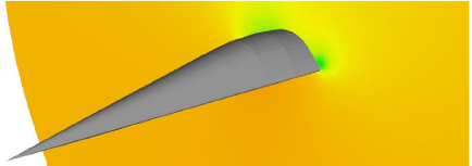
Failure to select the proper parent part(s) will result in an incorrect part being created. For example, if I intend to create a clip through the flow field on the geometry shown in the image below:
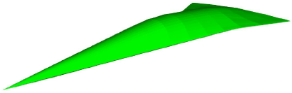
And I select the part representing the external flow field I will indeed see the clip I intend.
But if I instead select the surface part as the parent I will get:
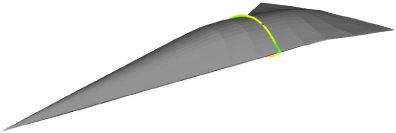
Both model parts and created parts can be parent parts. For example in the clip example above, if I wanted to view vector arrows on the clip part I would select the clip part as the parent.
See Parts for a complete list and description of derived parts that EnSight can create.
Auxiliary Geometry
Auxiliary geometry can be created around existing parts on which textures or images can be mapped, or shadows from the existing parts can be cast when exporting ray traced images. Various attributes of the geometry can be controlled such as, visible components, outline, thickness, double walls, etc. See Auxiliary Geometry.
Clips
A clip is a plane, line, box, ijk surface, xyz plane, rtz surface, quadric surface (cylinder, sphere, cone, etc.), or revolution surface passing through specified parent-parts. A clip can either be limited to a specific area (finite), or clip infinitely through the model. You control the location of the various clips with an interactive tool or appropriate parameter or coefficient input.
A clip line or plane will either be a true clip through the model, or can be made to be a grid where the grid density is under your control.
Clip surfaces can be animated as well as manipulated interactively.
In most cases you will create a clip which is the intersection of the clip tool and the parent parts. This clip can either be a true intersection or all elements that cross the intersection surface (a crinkly surface). You can also choose to cut the parent parts into half spaces.
See Clip Parts.
Contours
Contours are created by specifying which parts are to be contoured, and which variable to use. The contour levels can be tied to those of the palette or can be specified independently by the user.
See Contour Parts.
Developed Surfaces
Developed Surfaces can be created from cylindrical, spherical, conical, or revolution clip surfaces. You control the seam location and projection method that will flatten the surface.
Elevated Surfaces
Elevated Surfaces can be displayed using a scalar variable to elevate the displayed surface of specified parts. The elevated surface can have side walls.
Extrusions
Parts can be extruded to their next higher order. Namely a line can be extruded into a plane, a 2D surface into a 3D volume, etc. The extrusion can be rotational (such as would be desired for an axisymmetric part) or translational.
See Extruded Parts.
Isosurfaces
Isosurfaces can be created using a scalar, vector component, vector magnitude, or coordinate. Isosurfaces can be manipulated interactively or animated by incrementing the isovalue.
See Isosurface Parts
Particle Traces
Particle traces - both streamlines (steady state) and pathlines (transient) - trace the path of either a massless or massed particle in a vector field. You control which parts the particle trace will be computed through, the duration of the trace, which vector variable to use during the integration, and the integration time-step limits. Like other parts, the resulting particle trace part has nodes at which all of the variables are known, and therefore it can be colored by a different variable than the one used to create it. Components of the vector field can be eliminated by the user to force the trace to, for example, lie in a plane. The particle trace can either be displayed as a line, a ribbon, or a square tube showing the rotational components of the flow field. Streamlines can be computed upstream, downstream, or both.
Streamline and pathline particle traces originate from emitters, which you create. An emitter can be a point, rake, net, or can be the visible nodes of a part. Each emitter has a particle trace emit time specified which you set, and a re-emit time (if the data case is transient) can also be specified. Point, rake, and net emitters can be interactively positioned with the mouse. For streamlines, the particle trace continues to update as the emitter tool is positioned interactively by the user, or as the emitter part element boundary representation is updated.
Node track is another form of trace that is available. This trace is constructed by connecting the locations of nodes through time. It is useful for changing geometry or transient displacement models (including measured particles) which have node ids.
A further type of trace that is available is a min or max variable track. This trace is constructed by connecting the min or max of a chosen variable (for the selected parts) though time. Therefore, on transient models, one can follow where the min or max variable location occurs.
See Particle Trace Parts.
Points
Point parts are composed only of nodes. They can be created by reading an external file containing the xyz coordinates of the nodes, and/or by placing the cursor tool at desired locations and adding nodes. This feature can be used to essentially place probes in the model at particular locations. It can also be used to create parts that can be meshed with the 2D or 3D meshing capability within EnSight.
See Point Parts.
Profiles
Profile plots can be created by scalar, vector component, or vector magnitude. You control the orientation of the resulting profile plot.
See Profile Parts.
Separation/Attachment Lines
Separation and attachment lines show where flow abruptly leaves or returns to the 2D surface in 3D fields.
See Separation/Attachment Line Parts.
Shock Surfaces/Regions
Shock surfaces or regions show the location and extent of shock waves in a 3D flow field.
See Shock Regions/Surfaces Parts.
Subsets
A subset Part can contain node and element ranges of any model Part.
See Subset Parts.
Tensor Glyphs
Tensor glyphs show the direction of the principal eigenvectors. You specify which eigenvectors you wish to view and how you wish to view compression and tension.
See Tensor Glyph Parts.
Vector Arrows
Vector arrows show the direction and magnitude of a vector field. Vector arrows originate from element vertices, element nodes (including mid-side nodes), or from element centers. You specify which parts are to have arrows and which vector variable to use for the arrows, as well as a scale factor. You can eliminate components of the vector, and can also filter the arrows to eliminate high, low, low/high, or banded vector arrow magnitudes. The vector arrows can be either straight or curved, and can have arrow heads. The arrow heads are either proportional to the arrow or can be of fixed size.
See Vector Arrow Parts.
Vortex Cores
Vortex cores show the center of swirling flow in a flow field.
See Vortex Core Parts.
Part creation occurs on either the server or the client. Since the data that is available on the client and server are different, it is useful to understand where parts are created and where the resulting data is stored. By understanding this, you will understand why some parts can be created with certain parent parts and others cannot. For example, why you can't clip through a particle trace part (clips are created on the server and the particle trace part is not defined there). This information can be gained by examining the following table.
Table 1.1: Part Creation and Data Location
|
Part Type |
Where Created |
Data on Server |
Data on Client |
|---|---|---|---|
|
Clip |
Server |
Yes |
Depending on Element Rep |
|
Contour |
Client |
No |
Yes |
|
Developed Surface |
Server |
Yes |
Depending on Element Rep |
|
Elevated Surface |
Server |
Yes |
Depending on Element Rep |
|
Isosurface |
Server |
Yes |
Depending on Element Rep |
|
Material Part |
Server |
Yes |
Depending on Element Rep |
|
Particle Trace |
Server |
No |
Yes |
|
Point Part |
Server |
Yes |
Depending on Element Rep |
|
Profile |
Client |
No |
Yes |
|
Separation/Attachment Line |
Server |
Yes |
Depending on Element Rep |
|
Shock Surface/Region |
Server |
Yes |
Depending on Element Rep |
|
Subset |
Server |
Yes |
Depending on Element Rep |
|
Tensor Glyph |
Client |
No |
Yes |
|
Vector Arrow |
Client. Server if necessary. |
No |
Yes |
|
Vortex Core |
Server |
Yes |
Depending on Element Rep |
In the process of creating a part you will need to be able to select the parent part(s). This operation can be done from either the part list, the graphics window, or by key words from a search dialog.
See Select Parts.
The standard transformations of rotate, translate, and scale are available, as well as positioning of the Look-At and Look-From points and camera positions. The transformation-state (the specific view in the Graphics Window and Viewports) can be saved for later recall and use to a views manager. Transformations can be performed with precision in a dialog, or interactively with the mouse.
Normally transformations are performed on the entire scene. They can also be performed on a subset of the geometry (such as an exploded view). This is done by creating a coordinate frame and assigning part(s) to the new frame definition. The frame can be offset and rotated from the model axis system. Frames can have rectangular, cylindrical, or spherical coordinates.
Frames, and therefore all parts attached to them, can be periodic. Rotational or translational periodicity (as well as mirror symmetry) attributes are under user control allowing, for example, an entire pie to be built from one slice of the pie.
While parts are the fundamental entity in EnSight, the purpose of using EnSight is nearly always the pursuit of understanding the simulation results, that is, Variables.
Variables can either originate with the data file read or they can be computed using provided variables and geometry.
Variables can be defined on all nodes/elements or can be declared undefined for specified parts or node and element ranges.
Location
A field variable can be defined on an element center or at the vertices of the part.
Constant Variable
A Constant variable defines a single value and may
or may not be associated with any specific part. A Constant variable may
change value over time or be recomputed based on its parent parts. Total
Volume of a model is an example of a constant variable. It is often referred to
as a constant per case.
Constant Per Part Variable
A Constant Per Part variable defines a single value
for a given part. Each part can have its own value for the variable. It can change overtime.
Part Area would be a good example of a constant per part variable.
Note: Created parts will only inherit this variable if all parent parts have the same value.
Scalar Variable
A Scalar variable defines a single value for each
node or element on each part where it is defined. It creates a field of
data values. Temperature would be an example of a Scalar variable.
Vector Variable
A Vector variable defines three values -
representing the x, y, and z components of a vector - for each node or element on each part
where it is defined. It creates a field of data values. Velocity would
be an example of a Vector variable.
Tensor Variable
A Tensor variable defines nine values - representing
the components of a tensor - for each node or element on each part where it is defined. It
creates a field of data values. A stress tensor would be an example of
a Tensor variable.
Complex Scalars/Vectors
Scalar and Vector variables may
have a real and imaginary portion.
Variable Creation
New variables can be created either by specifying an equation via a calculator dialog or a predefined definition can be used. Similar to creating new parts, you will in most cases need to specify on what part(s) the new variable is computed. A large number of functions are currently available.
See Variable Creation.
In addition to visualizing information, you can make numerical queries.
You can query on information for a node, point, element, or a part.
You can query on information for a data set (such as size, number of elements, etc.)
You can query scalar and vector information for a point or node over time.
You can query scalar and vector information along a line. The line can either be a defined line in space, or a logical line composed of multiple 1D elements for a part (for example, query of a variable on a particle trace).
You can query to find the spatial or temporal mean as well as the min/max information for a variable.
Where applicable, query information can be in the form of a Fast Fourier Transform (FFT).
Plotting
The plotter plots Y vs. X curves. You control line style, axis control, line thickness and color. All query operations that result in multiple value output in EnSight can be sent to the plotter for display. You can control which curves to plot. Multiple curve plots are possible. All plottable query information can be saved to a disk file for use with other plotting packages.
See Query/Plotter and Interactive Probe Query.
EnSight handles transient (time dependent) data, including changing connectivity for the geometry. You can easily change between timesteps via the user interface. All parts and variables that are created, are updated to reflect the current display time (you can override this feature for individual parts). You can change to discrete step (called a timestep), or change to a time value (called continuous time) perhaps between two defined steps (EnSight will linearly interpolate between steps).
Note: Choosing the continuous option with changing connectivity will not interpolate between the steps (because this is impossible) but rather jump to the next timestep when its time value is reached.
CoProcessing
EnSight has the ability to update the number of timesteps dynamically
(that is, perhaps if the solver is in the process of writing the data and you are loading it
as the solution proceeds: CoProcessing). The only caveat is that EnSight needs a
never-to-exceed, maximum number of timesteps. This can be achieved by putting a
maximum time steps keyword in a Case Gold file, or in a
PLOT3D file, or by inserting a special routine (USERD_get_max_time_steps) into your user-defined
reader, indicating dynamically updating the number of timesteps may occur. See Advanced section of the Load Transient Data for details.
You can animate your model in four ways: particle trace animation, flipbook animation, solution time streaming, and keyframe animation.
Particle Trace Animation
Particle trace animation sends tracers down already created particle traces. You control the color, line type, speed and length of the animated traces.
If transient data is being animated at the same time, animated traces will automatically synchronize to the transient data time, unless you specifically indicate otherwise.
Flipbook Animation
A Flipbook animation reads in transient data, step by step, or moves a part spatially through a series of increments and stores the animation in memory. Playback is much faster as it requires no computation to move from frame to frame.
However, the trade-off is that Flipbook Animation can fill up your client memory. Flipbook animation is simpler to do than keyframe animation, while allowing four common types of animation:
Sequential presentation of transient data.
Mode shapes based on a nodal displacement variable.
EnSight created parts with an animation delta that recreates the part at a new location, that is, moving isosurfaces and Clip surfaces.
Sequential displacement by linear interpolation from zero to maximum vector value.
You can specify the display speed, and can step page-by-page through the animation in either direction. You can load some, or all the desired data. If you later load more data, you can choose to keep the already loaded data. With transient data, you can create pages between defined timesteps, with EnSight linearly interpolating the data.
Flipbooks can be created in two formats:
Object animation where new objects are created for each frame. You can then manipulate the model during animation play back.
Image animation where a bitmap image is created and stored for each animation page. For large models, image animation can sometimes take less memory - while trading off the capability to manipulate the model during animation.
See Flipbook Animation.
Solution Time Streaming
Solution time streaming accomplishes the same result as a flipbook animation of transient data except the data is never loaded into memory: it is streamed directly from disk one timestep at a time. While you don't see the animation speed of a flipbook, you only need enough memory to load in one step.
Keyframe Animation
Keyframe animation performs linearly interpolated transformations between specified key frames to create animation frames. Command language can be executed at key frames to script your animation. Some minimal editing is possible by deleting back to defined key frames. Animation key frames can be saved and restored from disk. Animation can be done on transient data and can automatically synchronize with simultaneous flipbook animation and particle trace animation.
Fly-around, rotate-objects, and exploded-view quick animations are predefined for easy use.
Keyframe animation can be recorded to disk files using a format of your choice.