


The MPC184 family of elements serves to connect the flexible and/or rigid components to each other in a multibody mechanism.
An MPC184 joint element is defined by two nodes with six degrees of freedom at each node (for a total of 12 DOFs). The relative motion between the two nodes is characterized by six relative degrees of freedom. Depending on the application, you can configure different kinds of joint elements by imposing appropriate kinematic constraints on any or some of these six relative degrees of freedom. For example, to simulate a revolute joint, the three relative displacement degrees of freedom and two relative rotational degrees of freedom are constrained, leaving only one relative degree of freedom available (the rotation around the revolute axis). Similarly, constraining the three relative displacement degrees of freedom and one relative rotational degree of freedom can simulate a universal joint. Two rotational degrees of freedom are "unconstrained" in this joint.
The kinematic constraints in joint elements are imposed using one of the following methods:
Lagrange multiplier method
Penalty-based method
The Lagrange multiplier method imposes the constraints more strictly than the penalty-based method. The number of degrees of freedom increases due to the additional Lagrange multipliers. Using the Lagrange multiplier method may result in an over-constrained system, therefore leading to convergence issues.
The penalty-based method does not increase the number of degrees of freedom in the model. However, the conditioning of the system matrices depends on the choice of penalty stiffness used in imposing these constraints. In general, the penalty method avoids the issues of over-constraint observed in the Lagrange multiplier method.
The following topics about using joint elements in a multibody analysis are available:
All joint elements are classified as MPC184 elements. The various elements are available via the MPC184 element's KEYOPT(1) setting and, in some cases, the KEYOPT(4) setting.
In addition, KEYOPT(2) determines the method for imposing the constraints:
| KEYOPT(2) = 0 invokes the Lagrange multiplier method (default) |
| KEYOPT(2) = 1 invokes the penalty-based method |
The following table lists the different types of joint elements and the required key option settings. The relevant element section in the Element Reference is also indicated.
| Joint Element Type | KEYOPT(1) | KEYOPT(4) | MPC184 Element | Constraints |
|---|---|---|---|---|
| Revolute | 6 | --- | Revolute Joint | 5 |
| Z-axis revolute | 6 | 1 | ||
| Universal | 7 | --- | Universal Joint | 4 |
| Slot | 8 | --- | Slot Joint | 2 |
| Point-in-plane | 9 | --- | Point-in-Plane Joint | 1 |
| Translational | 10 | --- | Translational Joint | 5 |
| Cylindrical | 11 | --- | Cylindrical Joint | 4 |
| Z-axis cylindrical | 11 | 1 | ||
| Spherical | 5 | --- | Spherical Joint | 3 |
| Planar | 12 | --- | Planar Joint | 3 |
| Z-axis planar | 12 | 1 | ||
| Weld | 13 | --- | Weld Joint | 6 |
| Orient | 14 | --- | Orient Joint | 3 |
| General | 16 | --- | General Joint |
Depends on number of fixed relative DOFs Minimum constraints = 0 (No DOF is fixed) Maximum constraints = 6 (All DOFs are fixed) |
| Screw | 17 | --- | Screw Joint | 5 Relative axial motion and rotational motion are linked via the pitch of the screw |
| Spotweld | 18 | --- | Spotweld Joint | None |
| Genb joint | 19 | --- | Genb Joint |
Depends on number of fixed relative DOFs Minimum constraints = 0 (No DOF is fixed) Maximum constraints = 6 (All DOFs are fixed) |
Following are some examples of joint element types:
Revolute Joint — Constrained degrees of freedom: UX, UY, UZ, ROTX, ROTY
 |
 |
Universal Joint — Constrained degrees of freedom: UX, UY, UZ, ROTY
 |
 |
Slot Joint — Constrained degrees of freedom: UY, UZ
 |
 |
Translational Joint — Constrained degrees of freedom: UY, UZ, ROTX, ROTY, ROTZ
|
|
|
Cylindrical Joint — Constrained degrees of freedom: UX, UY, ROTX, ROTY
 |
 |
Spherical Joint — Constrained degrees of freedom: UX, UY, UZ
 |
 |
Planar Joint — Constrained degrees of freedom: UZ, ROTX, ROTY
 |
 |
A joint element is typically defined by specifying two nodes, I and J. These nodes may be arbitrarily located in space. There are instances, however, when one of the nodes needs to be considered as a "grounded" node. In such cases, specify either node I or node J appropriately. In cases when the node is grounded, the location of the grounded node is taken to be that of the other specified node.
Example
If the first node of the joint element is a grounded node, then the element
definition is: E,,J or
EN,ElementNumber,,J
Similarly, if the second node is the grounded node, then the element
definition is: E,I, or
EN,ElementNumber,I
Each joint element must have an associated section definition. Issue SECTYPE to define the section type and subtype.
Example
The universal joint section definition is: SECTYPE,JOINT,UNIV,UNIV-01
Local coordinate systems at the nodes are required to define the kinematic constraints of a joint element. Issue SECJOINT to do so.
The local coordinate systems and their required orientation vary from one joint element to another. Input data requirements for each joint element differ. Typically, the local coordinate system is always defined at the first node of a joint element.
The local coordinate system at the second node may be optional. If it is not specified, then the local coordinate system at the first node is usually assumed.
The rotational components of the relative motion between the two nodes of the joint elements are quantified in terms of Bryant (or Cardan) angles that are evaluated based on these coordinate systems.
Example
The following figure illustrates the specification of the local coordinate system for a universal joint element:

Stops or limit constraints in joints are imposed on the available components of relative motion between the two nodes of a joint element. For static analysis, the stop constraints are based on the relative displacements (or relative rotations) of the free degrees of freedom.
Caution: Use joint stops sparingly. The program treats a stop constraint internally as a "must be imposed" or "hard" constraint, and no contact logic is used. As a result, during the given iteration of a substep, the stop constraints activate immediately if the program detects a violation of a stop limit.
Depending upon the nature of the problem, the stop constraint implementation may cause the solution to trend towards an equilibriated state that may not be readily apparent to you. In addition, do not use stops to simulate zero-displacement boundary conditions. You should also avoid specifying stops on multiple joints.
Finally, do not use joint stops as a substitute for contact modeling. Whenever possible, use node-to-node or node-to-surface contact modeling to simulate limit conditions.
Stops in Transient Dynamic Analysis
Stops are imposed based on the relative displacements (or rotations).
Lagrange Multiplier Method
In a transient dynamic analysis, if relative displacement-based (or rotation-based) stop constraints are used, then the relative velocities and relative accelerations become inconsistent (oscillatory velocity and/or accelerations are observed in many cases), implying that the energy and momentum due to the impact-like nature of the stops is not conserved. These inconsistencies are reasonably suppressed by imposing a numerical damping. However, numerical damping does not work appropriately in some cases. Thus, for the transient dynamic case, an energy-momentum conservation scheme is adopted. By this method, the user specified relative DOF stop values are taken into account, and constraints based on the relative velocity are imposed in such a way that the overall energy and momentum balance is achieved in a finite element sense.
Irrespective of the integration scheme specified for the transient dynamic analysis, the Newmark method is used for the joint element when stops are specified.
The energy-momentum conservation scheme for stops is implemented for all joints except the screw joint. In the case of the screw joint, the stops are imposed based on the relative displacements (or rotations).
The energy-momentum conservation scheme is not used when quasi-static simulation (TINTP,QUAS) is used in a transient dynamic analysis. Instead, the stops are implemented as regular inequality constraints.
Penalty-Based Method
The stops are implemented as regular inequality constraints in the penalty-based method. The energy-momentum conservation scheme is not used.
Defining Stops for Joint Elements
You can impose stops or limits on the available components of relative motion between the two nodes of a joint element. The stops or limits essentially constrain the values of the free degrees of freedom within a certain range. To specify minimum and maximum values, issue SECSTOP.
The following figure shows how stops can be imposed on a revolute joint such that the motion is constrained. The axis of the revolute is assumed to be perpendicular to the plane of paper and is along the e3 direction.

The local coordinate system specified at node I is assumed to be fixed in its initial configuration. However, the local coordinate system specified at node J evolves with the rotation of that node. The relative angle of rotation is given by:

Let the link with node J rotate with respect to the link with node I. This characteristic implies that the local coordinate system at node J rotates with respect to the local coordinate system at node I.
For the configuration shown, the initial relative angle of rotation is zero degrees. A counterclockwise motion results in positive angles of rotation. Clockwise motion results in negative angles of rotation.
If stops limit the movement of the link with node J (as shown), the stop conditions are specified as follows:
SECSTOP,6,
PHImin,PHImax
The next figure shows how stops can be imposed in a slot joint which involves displacements in the local eI 1 axis of node I. The relative distance between node J and node I is given by:

where xI and xJ are the
position vectors of nodes I and J. The initial distance between the nodes I and
J is l
0 and is a positive value.


Locks or locking limits may also be imposed on the available components of relative motion between the two nodes of a joint element. Locks are basically used in joint mechanisms to "freeze" the joint in a desired configuration during the course of deformation. When the locks are activated on a particular component of relative motion, that component remains locked for the rest of the analysis. Issue SECLOCK to define lock limits.
Referring to Figure 2.12: Stops Imposed on a Revolute Joint, the locks for a revolute
joint are specified as SECLOCK,6,
Phi_Min,Phi_Max
Referring to Figure 2.13: Stops Imposed on a Slot Joint, the locks for the slot
joint are specified as
SECLOCK,1,l_Min,l_Max
The following topics related to the material behavior of joint elements in a multibody analysis are available:
For more information, see MPC184 Joint in the Material Reference.
Linear or nonlinear stiffness and damping behavior can be associated with the
free or unrestrained components of relative motion of the joint elements. In the
case of linear stiffness or linear damping, the values are specified as
coefficients of a 6 x 6 elasticity matrix (TB,JOIN with
TBOPT = STIF or DAMP). The stiffness and damping
values can be temperature-dependent. Depending on the joint element in use, only
the appropriate coefficients of the stiffness or damping matrix are used in the
joint element constitutive calculations.
The nonlinear stiffness and damping behavior is specified via
TB,JOIN with an appropriate TBOPT
label. In the case of nonlinear stiffness, relative displacement (rotation)
versus force (moment) values are specified via TBPT. For
nonlinear damping behavior, velocity versus force behavior is specified via
TBPT. (See Figure 2.14: Nonlinear Stiffness and Damping Behavior for Joints for a
representation of the nonlinear stiffness or damping curve.) In either case,
these values may be temperature dependent; issue TBTEMP to
define the temperature for the data table.
The instantaneous slope (or stiffness/damping) and force value is determined from the user-specified curve. For instance, if the current data point (displacement/velocity) falls between two user-specified points, the slope and force at that point is determined from those two user-specified points. However, if the current data point falls on a user-defined point, the force is obtained from that point while the slope is approximated by the line joining the data points behind and ahead of the current data point.

You can specify the linear or nonlinear stiffness or damping behavior independently for each component of relative motion. However, if you specify linear stiffness for an unrestrained component of relative motion, you cannot specify nonlinear stiffness behavior on the same component of relative motion. The damping behavior is similarly restricted. If a joint element has more than one free or unrestrained component of relative motion--for example, the universal joint has two free components of relative motion--then you can independently specify the stiffness or damping behavior as linear or nonlinear for each of the unrestricted components of relative motion.
Frictional behavior along the unrestrained components of relative motion
influences the overall behavior of the joints. You can model Coulomb friction
for joint elements via TB,JOIN with an appropriate
TBOPT label. Frictional behavior can be specified
only for the following joints:
| Revolute Joint (x-axis and z-axis) |
| Slot Joint |
| Translational Joint |
| Spherical Joint |
The laws governing the frictional behavior of the joint are described below.
Coulomb’s Law
The classical Coulomb friction model is implemented for joints using a penalty formulation. The Coulomb friction model for joints is defined as:


Where, F s is the equivalent tangential force (or moment), F n is the normal force (or moment) in the joint, and μ is the current value of the coefficient of friction. The calculation of the normal force depends on the joint under consideration.
If the equivalent tangential force F s is less than F lim , the state is known as the sticking state. If F s exceeds F lim , sliding occurs and the state is known as the sliding state. The sticking/sliding calculations determine when a point transitions from sticking to sliding or vice versa.

Exponential Friction Law
The exponential friction law is used to smooth the transition between the static coefficient of friction and the dynamic coefficient of friction according to the formula (Benson and Hallquist):

where:
V rel = the relative slip rate
μ s = the coefficient of friction in the static regime (stiction)
μ d = the coefficient of friction in the dynamic regime
c = decay coefficient

The modeling of Coulomb friction in joints requires some geometry specifications, depending on the type of joint under consideration. These quantities are used in the computation of the normal force (or moment) for Coulomb friction calculations (SECJOINT).
The following table outlines the required geometric quantities:
Table 2.2: Required Geometric Quantities
| Joint Type | Geometric Quantities |
| Revolute Joint (x-axis and z-axis) | Outer radius, Inner radius, Effective Length |
| Slot Joint | None required |
| Translational Joint | Effective Length, Effective Radius |
| Spherical Joint | Effective Radius |
If appropriate geometric quantities are not specified, then the corresponding normal force contributions will not be considered. The following section explains the normal force calculations and the geometric quantities required.
The normal force (or moment) that is used in the Coulomb frictional behavior is based on the following forces that arise in a joint:
Constraint forces (or moments) - Lagrange multiplier forces or penalty constraint forces
Interference fit forces (or moments)
The descriptions here assume the Lagrange multiplier method, but the same ideas hold true for the penalty-based joint element implementation.
Revolute Joint
In order to compute the normal moment in a revolute joint, the revolute joint is visualized as a cylinder-pin assembly (for example, a door hinge consisting of a pin with a head inserted into a cylinder).
The following geometric quantities are required in the calculations below. Note that the specification of these quantities is optional. If some of these geometric quantities are not specified, then the corresponding contribution to the normal moment calculations is ignored.
R outer = Outer radius of the cylinder
R inner = Inner radius of the cylinder or outside radius of pin
L eff = The effective length is the length over which the cylinder and pin are in contact with each other
The contributions to the normal moment in an x-axis revolute joint are as follows:
An axial moment due to the axial component of the constraint Lagrange multiplier force (λ1 ).
This force acts in such a way as to push the cylinder against the pin head, thereby causing a frictional moment to develop.
where,
A tangential moment due to the constraint Lagrange multiplier forces, λ2 and λ3:
A bending moment that is generated as a consequence of the constraint Lagrange multiplier moments (λ5 and λ6):
Leading to a bending moment:


Additionally, if interference fit moment (M interference ) is defined, the normal moment for frictional calculations is given by:

A similar calculation is carried out for the z-axis revolute joint by choosing the appropriate constraint Lagrange multiplier forces in the above equations.
Slot Joint
The two displacement constraint Lagrange multiplier forces (λ2 and λ3) in the slot joint contribute to a tangential force as follows:

Additionally, if interference fit force (F interference ) is defined, the normal force for frictional calculations is given by:

Geometric quantities are not required for the slot joint.
Translational Joint
The geometric quantities required for the translation joint are:
L eff = Effective length. The effective length is the length over which the two parts of the translation joint overlap. It is assumed that the change in this length is small.
R eff = Effective radius. To simplify calculations, an effective radius is used in torsional moment calculations, even though the cross section in a translational joint is rectangular. The effective radius is used in computing the force that arises due to the torsional moment.
The normal force used in frictional calculations is computed as follows:
An effective radial force due to the constraint forces (λ2 and λ3):
Bending force due to in-plane constraint moments (λ5 and λ6):
Leading to a bending force
Force due to the torsional constraint moment, λ4:


Additionally, if interference fit force (F interference ) is defined, the normal force for frictional calculations is given by:

Spherical Joint
The geometric quantity required for the spherical joint is:
R eff = Effective radius. The effective radius is the radius at which the inner sphere contacts the outer sphere of the spherical joint. The gap between the two spheres is not considered for frictional calculations.
For frictional calculations, the instantaneous axis of rotation is calculated as:

where:
 = angular velocity of body J = angular velocity of body J |
 = angular velocity of body I = angular velocity of body I |
 = time increment = time increment |
The normal moment arises due to the constraint forces as follows:


The friction parameters are defined using the
TB,JOIN,,,,TBOPT command.
The following table outlines the available TBOPT
settings.
Table 2.3: Required Geometric Quantities
| Joint Type |
Available
TBOPT Labels
|
| Revolute Joint (x-axis) | MUS4, EXP4, SL4, SK4, FI4 |
| Revolute Joint (z-axis) | MUS6, EXP6, SL6, SK6, FI6 |
| Slot Joint | MUS1, EXP1, SL1, SK1, FI1 |
| Translational Joint | MUS1, EXP1, SL1, SK1, FI1 |
| Spherical Joint | MUS6, SL6, SK6 |
For more information, see the TB command and Frictional Behavior in the Material Reference.
The initial configuration of the joint element may be such that nonzero forces or moments is necessary. In such cases, you can define the constitutive behavior with respect to a reference configuration such that these forces or moments are zero. To do so, define a "reference angle" or a "reference length" (SECDATA).
If you do not define reference lengths and angles, Mechanical APDL calculates the values from the initial configuration of the joints. The program uses the reference lengths and angles in the stiffness and frictional behavior calculations.
Issue the DJ command to impose boundary conditions on the available components of relative motion of the joint element. You can list the imposed values via the DJLIST command. To delete the values, issue the DJDELE command.
To apply concentrated forces on the available components of relative motion of the joint element, issue the FJ command. You can list the imposed values via the FJLIST command. To delete the values, issue the FJDELE command.
Other than in idealized geometry (such as that shown in Figure 2.1: FE Slider-Crank Mechanism ), an MPC184 joint element is defined by one or two nodes in space and requires special modeling techniques to connect the joint to the body appropriately.
Figure 2.17: Pinned Joint Geometry shows a 3D model of a pinned joint where the geometry of the joint (the pin) is explicitly modeled. To perform a multibody analysis, the pin geometry is ignored and the behavior replaced by the appropriate MPC184 joint element.
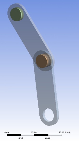
Figure 2.18: Pinned Joint Mesh and Revolute Joint shows the meshed model including the revolute joint. To connect the bodies to the joint, you must use either elements (such as beams) or constraint equations. The easiest way to do so is to use contact elements to create surface-based constraints (multipoint constraints, or MPCs), as follows:
Define a pilot node at one end of the joint. The pilot node connects the joint to the rest of the body.
Select the nodes on the surface of the body that you want to connect to this pilot node.
Create contact surface elements on this surface. By sharing the same real constant number (REAL,
N), MPCs between the surface nodes and the pilot node are generated during the solution.
Repeat the steps for each body-joint connection.
Figure 2.19: Pinned Joint Contact Elements shows the contact elements and Figure 2.20: Pinned Joint Constraint Equations shows the MPCs (constraint equations) created during the solution for the lower body.
Create the pilot node using the TARGE170 element--setting KEYOPT(2) = 1 so as not to allow the program to constrain any DOFs--and issuing the TSHAP,PILO command.
Use CONTA174 as the element type for the surface mesh. Set the following contact element key options to create the necessary constraints:
| KEYOPT(2) = 2 | Constraint (MPC) option. |
| KEYOPT(4) = 2 | Generate rigid MPC constraints. |
| KEYOPT(12) = 5 | Bonded behavior between the pilot node and the contact surface. |
Instead of the rigid option, you can also choose a flexible (force-distributed or RBE3-type) constraint option by setting KEYOPT(4) = 1. The following figures illustrate the difference in behaviors:


Typical Command Sequence
Following is a typical command sequence for connecting bodies to joints:
! Step 1: Define a pilot node at the joint node
et,59,170          ! type ID=59 is an available ID
keyopt,59,2,1      ! do not allow program to constrain DOFs
real,59            ! real ID=59 is an available ID
tshap,pilot
e,9536             ! "9536" is the joint node
! Step 2: Select the nodes of the corresponding surface
csys,15            ! CS at center of pin
nsel,s,loc,x,15    ! nodes at r=15
! Step 3: Create the contact elements on the surface
et,60,174
keyopt,60,2,2      ! constraint (MPC) option
keyopt,60,4,2      ! rigid MPC
keyopt,60,12,5     ! bonded always contact
type,60
real,59            ! same real ID: this connects the pilot
                   !   to this surface
esurf              ! generate the contact elements on the surface
nsel,all
Additional Information
For more information about using contact elements to generate constraints, see Surface-Based Constraints in the Contact Technology Guide.