


SOLID278
3D 8-Node
Thermal Solid
SOLID278 Element Description
SOLID278 has a 3D thermal conduction capability. The element has eight nodes with a single degree of freedom, temperature, at each node. The element is applicable to a 3D, steady-state or transient thermal analysis. The element can also account for heat transfer by a mass flow with a prescribed velocity field (see Mass Transport (Advection) in the Theory Reference). If the model containing the conducting solid element is also to be analyzed structurally, the element should be replaced by an equivalent structural element (such as SOLID185). See SOLID279 for a similar thermal element, with mid-edge node capability. For more details about this element, see SOLID278 - 3D 8-Node Homogeneous/Layered Thermal Solid in the Theory Reference.
SOLID278 is available in these forms:
Homogeneous Thermal Solid (KEYOPT(3) = 0, the default) -- See "SOLID278 Homogeneous Thermal Solid Element Description".
Layered Thermal Solid (KEYOPT(3) = 1), or Layered Thermal Solid with through-the-thickness degrees of freedom (KEYOPT(3) = 2) -- See "SOLID278 Layered Thermal Solid Element Description".
See SOLID278 in the Mechanical APDL Theory Reference for more details about this element.
A higher-order version of the SOLID278 element is SOLID279.
SOLID278 Homogeneous Thermal Solid Element Description
SOLID278 Thermal Solid is suitable for modeling general 3D solid heat conduction. It allows for prism and tetrahedral degenerations when used in irregular regions. SOLID278 is designed to be a companion element for SOLID185.

SOLID278 Homogeneous Thermal Solid Input Data
The geometry and node locations for this element are shown in Figure 278.1: SOLID278 Homogeneous Thermal Solid Geometry. The element is defined by eight nodes and the orthotropic material properties. The default element coordinate system is along global directions. You may define an element coordinate system using ESYS, which forms the basis for orthotropic material directions (namely, for thermal conductivity). Specific heat and density are ignored for steady-state solutions. Properties not input default as described in the Material Reference.
As described in Coordinate Systems, you can use ESYS to orient the material properties and the temperature gradient and heat flux output. Use RSYS to choose output that follows the material coordinate system or the global coordinate system.
Element loads are described in Element Loading. Convection or heat flux (but not both) and radiation may be input as surface loads at the element faces as shown by the circled numbers on Figure 278.1: SOLID278 Homogeneous Thermal Solid Geometry. Heat generation rates may be input as element body loads at the nodes. If the node I heat generation rate HG(I) is input, and all others are unspecified, they default to HG(I).
A mass transport option is available with KEYOPT(11). With this option, you specify the velocity components VX, VY, and VZ by issuing BF,,VELO,VX,VY, VZ. There is no restriction on the element Peclet number (Pe) for this element, and it offers the Streamline Upwind Petrov-Galerkin (SUPG) formulation and Discontinuity Capturing (DC) terms that enable convergence for high Pe conditions (see Galerkin or Streamline Upwind Petrov-Galerkin (SUPG) Formulation in the Thermal Analysis Guide). You can control the settings that activate the SUPG formulation and include one of three DC terms to smooth spurious oscillations if they arise in your solution by setting real constants with the R and RMORE commands as detailed in the table below. With mass transport, temperatures should be specified along the entire inlet boundary to assure a stable solution, and you should use specific heat (C) and density (DENS) material properties instead of enthalpy (ENTH). For more detais, see Mass Transport (Advection) in the Theory Reference and Mass Transport (Advection) in the Thermal Analysis Guide.
"SOLID278 Homogeneous Thermal Solid Input Summary" contains a summary of element input. For a general description of element input, see Element Input.
SOLID278 Homogeneous Thermal Solid Input Summary
- Nodes
I, J, K, L, M, N, O, P
- Degrees of Freedom
TEMP
- Real Constants
Real Constants Used for Mass Transport (if KEYOPT (11) = 1 or 2) to Activate the Streamline Upwind Petrov-Galerkin (SUPG) Formulation and One of Three Discontinuity Capturing (DC) Terms [a] No. [b] Name Default [c] Description 2 SUPG1.0 Acts as a multiplier on the stabilizing term of the SUPG formulation and enables you to choose also a DC term to smooth oscillations. To activate the Galerkin Formulation, use a small number(1.e-12), as an exact zero value reverts back to 1.0 internally and enables SUPG formulation.
3 TGRADMAG1.0e-6 Thermal gradient threshold value, above which the DC term that you select will be applied. If the thermal gradient is less than the value you specify for TGRADMAG, the DC term is not applied, and vice versa, if it is greater, the nonlinear stabilizing DC term will be applied.5 DC1[d]0.0 Any non-zero value (typically 1.0) selects the DC1 term to be added to your analysis and acts as a multiplier on this stabilizing term. 6 DC2[d]0.0 Any non-zero value (typically 1.0) selects the DC2 term to be added to your analysis and acts as a multiplier on this stabilizing term. 7 DC3[d]0.0 Any non-zero value (typically 1.0) selects the DC3 term to be added to your analysis and acts as a multiplier on this stabilizing term. [a] The SUPG formulation and DC terms can be used to smooth oscillations that can occur for flow conditions with high Pe. For details, see Galerkin or Streamline Upwind Petrov-Galerkin (SUPG) Formulation in the Thermal Analysis Guide.
[c] If you do not specify any real constants, the mass transport solution will be based on the SUPG formulation without any DC terms.
[d] Activating more than one DC term at a time will produce an error message.
- Material Properties
TB command: See Element Support for Material Models for this element. MP command: KXX, KYY, KZZ, DENS, C, ENTH - Surface Loads
- Convection or Heat Flux (but not both) and Radiation (using Lab = RDSF) --
face 1 (J-I-L-K), face 2 (I-J-N-M), face 3 (J-K-O-N), face 4 (K-L-P-O), face 5 (L-I-M-P), face 6 (M-N-O-P)
- Body Loads
- Velocity for Mass Transport (KEYOPT(11) = 1 or 2) --
Specify the velocity components VX, VY, and VZ by issuing BF,,VELO,VX,VY,VZ
- Special Features
- KEYOPT(2)
Evaluation of film coefficient:
- 0 --
Evaluate film coefficient (if any) at average film temperature, (TS + TB)/2
- 1 --
Evaluate at element surface temperature, TS
- 2 --
Evaluate at fluid bulk temperature, TB
- 3 --
Evaluate at differential temperature |TS-TB|
- KEYOPT(3)
Layer construction:
- 0 --
Homogeneous Solid (default) -- Nonlayered
- KEYOPT(9)
Element-level matrix form:
- 0 --
Symmetric (default)
- 1 --
Nonsymmetric
- KEYOPT(11)
Mass transport effects:
- 0 --
Do not include mass transport in the analysis.
- 1 --
Include mass transport with Diffusive Flux (Dflux) Neumann boundary condition. You may want to choose the Dflux Neumann boudary condition if you are not interested in an energy balance as it is easier to specify compared to the Tflux boundary condition (see Diffusive Flux and Total Flux Neumann Boundary Conditions in the Theory Reference for details).
- 2 --
Include mass transport with Total Flux (Tflux) Neumann boundary condition. The Tflux Neumann boundary condition will satisfy an energy balance with the PRRSOL command, but setting up its Neumann boundary condition is slightly more complex than the Dflux option (see Diffusive Flux and Total Flux Neumann Boundary Conditions in the Theory Reference for details).
Note: Do not create models that have some elements with a value of 1 and others with a value of 2 for KEYOPT(11). On the other hand, it is possible to have combinations of elements with KEYOPT(11) = 0 and 2 as well as KEYOPT(11) = 0 and 1 in the same model.
- KEYOPT(13)
Film coefficient matrix:
- 0 --
Program determines whether to use a diagonal or consistent film coefficient matrix.
- 1 --
Use a diagonal film coefficient matrix (default).
- 2 --
Use a consistent matrix for the film coefficient.
- KEYOPT(15)
Specific heat matrix:
- 0 --
Program determines whether to use a diagonal or consistent specific heat matrix (default). For details on default behavior, see SOLID278 Homogeneous Thermal Solid Assumptions and Restrictions.
- 1 --
Use a diagonal specific heat matrix.
- 2 --
Use a consistent specific heat matrix.
- KEYOPT(16)
Evaluation of material properties:
- 0 --
Evaluate material properties at centroid (default).
- 1 --
Evaluate material properties at each integration point.
Note: If THOPT,QUASI has been issued, KEYOPT(16) is ignored and material properties are evaluated at the centroid.
SOLID278 Homogeneous Thermal Solid Output Data
The solution output associated with the element is in two forms:
Nodal temperatures included in the overall nodal solution
Additional element output as shown in Table 278.1: SOLID278 Homogeneous Thermal Solid Output Definitions
Output temperatures may be read by structural solid elements (such as SOLID185 and SOLSH190) via the LDREAD,TEMP command.
Convection heat flux is positive out of the element; applied heat flux is positive into the element.
The element output directions are parallel to the element coordinate system.
A general description of solution output is given in Solution Output. See the Basic Analysis Guide for ways to view results.
The Element Output Definitions table uses the following notation:
A colon (:) in the Name column indicates that the item can be accessed by the Component Name method (ETABLE, ESOL). The O column indicates the availability of the items in the file jobname.out. The R column indicates the availability of the items in the results file.
In either the O or R columns, “Y” indicates that the item is always available, a letter or number refers to a table footnote that describes when the item is conditionally available, and “-” indicates that the item is not available.
Table 278.1: SOLID278 Homogeneous Thermal Solid Output Definitions
| Name | Definition | O | R |
|---|---|---|---|
| EL | Element Number | Y | Y |
| NODES | Nodes - I, J, K, L, M, N, O, P | Y | Y |
| MAT | Material number | Y | Y |
| VOLU: | Volume | Y | Y |
| XC, YC, ZC | Location where results are reported | Y | 2 |
| HGEN | Heat generations HG(I), HG(J), HG(K), HG(L), HG(M), HG(N), HG(O), HG(P) | Y | - |
| TG:X, Y, Z | Thermal gradient components | Y | Y |
| TF:X, Y, Z | Thermal flux (heat flow rate/cross-sectional area) components | Y | Y |
| FACE | Face label | 1 | - |
| AREA | Face area | 1 | 1 |
| NODES | Face nodes | 1 | - |
| HFILM | Film coefficient at each node of face | 1 | - |
| TBULK | Bulk temperature at each node of face | 1 | - |
| TAVG | Average face temperature | 1 | 1 |
| HEAT RATE | Heat flow rate across face by convection | 1 | 1 |
| HEAT RATE/AREA | Heat flow rate per unit area across face by convection | 1 | - |
| HFAVG | Average film coefficient of the face | - | 1 |
| TBAVG | Average face bulk temperature | - | 1 |
| HFLXAVG | Heat flow rate per unit area across face caused by input heat flux | - | 1 |
| HFLUX | Heat flux at each node of face | 1 | - |
Available only at centroid as a *GET item.
Table 278.2: SOLID278 homogeneous Thermal Solid Item and Sequence Numbers lists output available via ETABLE using the Sequence Number method. See Element Table for Variables Identified By Sequence Number in the Basic Analysis Guide and The Item and Sequence Number Table in this reference for more information. The following notation is used in Table 278.2: SOLID278 homogeneous Thermal Solid Item and Sequence Numbers:
- Name
output quantity as defined in the Table 278.1: SOLID278 Homogeneous Thermal Solid Output Definitions
- Item
predetermined Item label for ETABLE command
- FCn
sequence number for solution items for element Face n
SOLID278 Homogeneous Thermal Solid Assumptions and Restrictions
Zero-volume elements are not allowed.
Elements may be numbered either as shown in Figure 278.1: SOLID278 Homogeneous Thermal Solid Geometry or may have the planes IJKL and MNOP interchanged. The element may not be twisted such that the element has two separate volumes (which occurs most frequently when the elements are not numbered properly).
All elements must have eight nodes. You can form a prism-shaped element by defining duplicate K and L and duplicate O and P node numbers. (See Degenerated Shape Elements.) A tetrahedron shape is also available.
If the thermal element is to be replaced by a SOLID185 structural element with surface stresses requested, the thermal element should be oriented such that face I-J-N-M and/or face K-L-P-O is a free surface.
A free surface of the element (that is, not adjacent to another element and not subjected to a boundary constraint) is assumed to be adiabatic.
The full Newton-Raphson solution option (THOPT,FULL) must be used if thermal properties are defined via TB,THERM.
If enthalpy is defined, density and specific heat will be ignored.
The default for KEYOPT(15) depends on whether or not mass transport is included in the analysis:
If mass transport is not included in the analysis (KEYOPT (11) = 0), the default is to use a diagonal specific heat matrix. If mass transport is included in the analysis (KEYOPT (11) = 1 or 2), the default is to use a consistent specific heat matrix.
This element is available in layered form. See "SOLID278 Layered Thermal Solid Assumptions and Restrictions".
SOLID278 Layered Thermal Solid Element Description
Use SOLID278 Layered Thermal Solid
to model heat conduction in layered thick shells or solids. The layered
section definition is given by section (SECxxx) commands. A prism degeneration option is also available.
Figure 278.2: SOLID278 Layered Thermal Solid Geometry

xo = Element x-axis if ESYS is not specified.
x = Element x-axis if ESYS is specified.
SOLID278 Layered Thermal Solid Input Data
The geometry and node locations for this element are shown in Figure 278.2: SOLID278 Layered Thermal Solid Geometry. The element is defined by eight nodes. A prism-shaped element may be formed by defining the same node numbers for nodes K and L, and O and P.
In addition to the nodes, the element input data includes the anisotropic material properties. Anisotropic material directions correspond to the layer coordinate directions which are based on the element coordinate system. The element coordinate system follows the shell convention where the z axis is normal to the surface of the shell. The nodal ordering must follow the convention that I-J-K-L and M-N-O-P element faces represent the bottom and top shell surfaces, respectively. You can change the orientation within the plane of the layers via the SECDATA command in the same way that you would for shell elements (as described in Coordinate Systems). To achieve the correct nodal ordering for a volume mapped (hexahedron) mesh, you can use the VEORIENT command to specify the desired volume orientation before executing the VMESH command. Alternatively, you can use the EORIENT command after automatic meshing to reorient the elements to be in line with the orientation of another element, or to be as parallel as possible to a defined ESYS axis.
Layered Section Definition Using Section Commands
You can associate SOLID278 Layered Solid with a shell section
(SECTYPE). The layered composite specifications (including layer
thickness, material, orientation, and number of integration points through the thickness of
the layer) are specified via shell section (SECxxx) commands. You
can use the shell section commands even with a single-layered element. Mechanical APDL obtains the
actual layer thicknesses used for element calculations by scaling the input layer thickness so
that they are consistent with the thickness between the nodes.
You can designate the number of integration points (1, 3, 5, 7, or 9) located through the thickness of each layer. Two points are located on the top and bottom surfaces respectively and the remaining points are distributed equal distance between the two points. The element requires at least two points through the entire thickness. When no shell section definition is provided, the element is treated as single-layered and uses two integration points through the thickness.
SOLID278 Layered Thermal Solid does not support real constant input for defining layer sections.
SOLID278 Layered
Thermal Solid has an option for through-the-thickness degrees of freedom
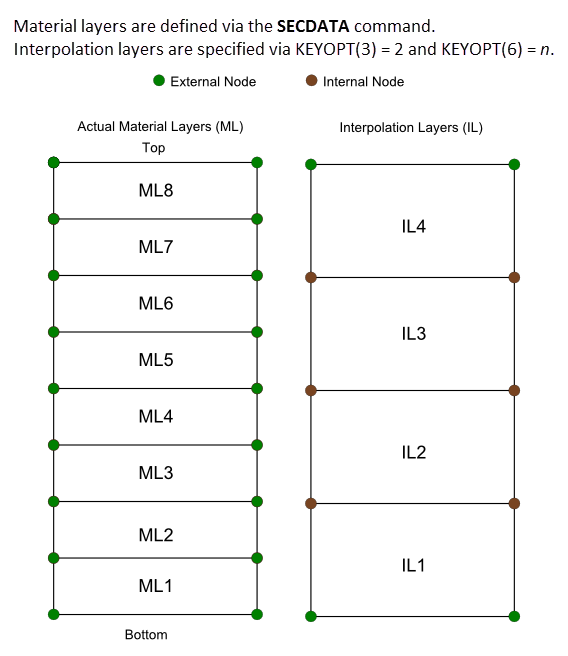
(KEYOPT(3) = 2). As shown in Figure 278.3: Understanding Interpolation Layers,
the option works by creating a specified number of material layers
(defined via the SECDATA command) per interpolation
layer (KEYOPT(6) = n). Each interpolation
layer has four internal nodes,
one on each face. KEYOPT(3) = 2 offers greater accuracy than KEYOPT(3)
= 1 but is more computationally intensive; the more material layers
specified per interpolation layer, the greater the accuracy and computational
cost.
Other Input
The default orientation for this element has the S1 (shell surface coordinate) axis aligned with the first parametric direction of the element at the center of the element and is shown as xo in Figure 278.2: SOLID278 Layered Thermal Solid Geometry.
The default first surface direction S1 can be reoriented in the element reference plane (as shown in Figure 278.2: SOLID278 Layered Thermal Solid Geometry) via the ESYS command. You can further rotate S1 by angle THETA (in degrees) for each layer (via the SECDATA command) to create layer-wise coordinate systems. See Coordinate Systems for details.
The geometry, node locations, and the coordinate system for this element are shown in Figure 278.2: SOLID278 Layered Thermal Solid Geometry. The element is defined by eight nodes and the orthotropic material properties. A prism-shaped element may also be formed as shown in Figure 278.2: SOLID278 Layered Thermal Solid Geometry. Orthotropic material directions correspond to the layer coordinate directions. The element coordinate system orientation is as described in Coordinate Systems. Specific heat and density are ignored for steady-state solutions. Properties not input default as described in the Material Reference.
Element loads are described in Element Loading. Convection or heat flux (but not both) and radiation may be input as surface loads at the element faces as shown by the circled numbers on Figure 278.2: SOLID278 Layered Thermal Solid Geometry. Heat generation rates may be input as element body loads on a per layer basis. One heat generation value is applied to the entire layer. If the first layer heat generation rate HG(1) is input, and all others are unspecified, they default to HG(1).
The following table summarizes the element input. Element Input provides a general description of element input.
SOLID278 Layered Thermal Solid Input Summary
- Nodes
I, J, K, L, M, N, O, P
- Degrees of Freedom
TEMP
- Material Properties
TB command: See Element Support for Material Models for this element. MP command: KXX, KYY, KZZ, DENS, C - Surface Loads
- Convection or Heat Flux (but not both) and Radiation (using Lab = RDSF) --
face 1 (J-I-L-K), face 2 (I-J-N-M), face 3 (J-K-O-N), face 4 (K-L-P-O), face 5 (L-I-M-P), face 6 (M-N-O-P)
- Body Loads
- Heat Generations --
HG(1), HG(2), HG(3), . . . , HG(number of layers)
For the layered solid (KEYOPT(3) = 1 or 2), heat generation can be defined with the BFE command only.
- Special Features
- KEYOPT(2)
Evaluation of film coefficient:
- 0 --
Evaluate film coefficient (if any) at average film temperature, (TS + TB)/2
- 1 --
Evaluate at element surface temperature, TS
- 2 --
Evaluate at fluid bulk temperature, TB
- 3 --
Evaluate at differential temperature |TS-TB|
- KEYOPT(3)
Layer construction:
- 1 --
Layered Solid
- 2 --
Layered Solid with through-the-thickness degrees of freedom
- KEYOPT(6)
Number of material layers (>= 1) per interpolation layer (valid only when KEYOPT(3) = 2):
- 1 --
Single material layer per interpolation layer (default)
-
n-- nmaterial layers per interpolation layer
- KEYOPT(8)
Material layer data storage:
- 0 --
Store data for bottom of bottom layer and top of top layer (default)
- 1 --
Store top and bottom data for all layers. (The volume of data may be considerable.)
- KEYOPT(9)
Element-level matrix form:
- 0 --
Symmetric (default)
- 1 --
Nonsymmetric
- KEYOPT(13)
Film coefficient matrix:
- 0 --
Program determines whether to use a diagonal or consistent film coefficient matrix.
- 1 --
Use a diagonal film coefficient matrix (default).
- 2 --
Use a consistent film coefficient matrix.
- KEYOPT(15)
Specific heat matrix:
- 0 --
Program determines whether to use a diagonal or consistent specific heat matrix.
- 1 --
Use a diagonal specific heat matrix (default).
- 2 --
Use a consistent specific heat matrix.
SOLID278 Layered Thermal Solid Output Data
The solution output associated with the element is in two forms:
Nodal temperatures included in the overall nodal solution
Additional element output as shown in Table 278.3: SOLID278 Layered Thermal Solid Element Output Definitions
Output temperatures may be read by structural solid elements (such as SOLID185 and SOLSH190) via the LDREAD,TEMP command.
Figure 278.4: SOLID278 Layered Thermal Solid Heat Flux/Temperature Gradient Output

Heat flux directions shown are for global directions.
Convection heat flux is positive out of the element; applied heat flux is positive into the element.
The element output directions are parallel to the layer coordinate system.
A general description of solution output is given in Solution Output. See the Basic Analysis Guide for ways to view results.
To see the temperature distribution through the thickness for this element, enter the POST1 postprocessor (/POST1), then issue /GRAPHICS,POWER and /ESHAPE,1 followed by PLESOL,BFE,TEMP
The Element Output Definitions table uses the following notation:
A colon (:) in the Name column indicates that the item can be accessed by the Component Name method (ETABLE, ESOL). The O column indicates the availability of the items in the file jobname.out. The R column indicates the availability of the items in the results file.
In either the O or R columns, “Y” indicates that the item is always available, a letter or number refers to a table footnote that describes when the item is conditionally available, and “-” indicates that the item is not available.
Table 278.3: SOLID278 Layered Thermal Solid Element Output Definitions
| Name | Definition | O | R |
|---|---|---|---|
| EL | Element Number | Y | Y |
| NODES | Nodes - I, J, K, L, M, N, O, P | Y | Y |
| MAT | Material number | Y | Y |
| VOLU: | Volume | Y | Y |
| XC, YC, ZC | Location where results are reported | Y | 2 |
| HGEN | Heat generations HG(1), HG(2), HG(3), . . . | Y | - |
| TG:X, Y, Z | Thermal gradient components | Y | Y |
| TF:X, Y, Z | Thermal flux (heat flow rate/cross-sectional area) components | Y | Y |
| FACE | Face label | 1 | - |
| AREA | Face area | 1 | 1 |
| NODES | Face nodes | 1 | - |
| HFILM | Film coefficient at each node of face | 1 | - |
| TBULK | Bulk temperature at each node of face | 1 | - |
| TAVG | Average face temperature | 1 | 1 |
| HEAT RATE | Heat flow rate across face by convection | 1 | 1 |
| HEAT RATE/AREA | Heat flow rate per unit area across face by convection | 1 | - |
| HFAVG | Average film coefficient of the face | - | 1 |
| TBAVG | Average face bulk temperature | - | 1 |
| HFLXAVG | Heat flow rate per unit area across face caused by input heat flux | - | 1 |
| HFLUX | Heat flux at each node of face | 1 | - |
Available only at centroid as a *GET item.
Table 278.4: SOLID278 Layered Thermal Solid Item and Sequence Numbers lists output available via ETABLE using the Sequence Number method. See Element Table for Variables Identified By Sequence Number in the Basic Analysis Guide and The Item and Sequence Number Table in this reference for more information. The following notation is used in Table 278.4: SOLID278 Layered Thermal Solid Item and Sequence Numbers:
- Name
output quantity as defined in Table 278.3: SOLID278 Layered Thermal Solid Element Output Definitions
- Item
predetermined Item label for ETABLE command
- FCn
sequence number for solution items for element Face n
SOLID278 Layered Thermal Solid Assumptions and Restrictions
Zero-volume elements are not allowed.
Elements may be numbered either as shown in Figure 278.2: SOLID278 Layered Thermal Solid Geometry or may have the planes IJKL and MNOP interchanged. The element may not be twisted such that the element has two separate volumes (which occurs most frequently when the elements are not numbered properly).
All elements must have eight nodes. You can form a prism-shaped element by defining duplicate K and L and duplicate O and P node numbers. (See Degenerated Shape Elements.)
If the thermal element is to be replaced by a SOLID185 structural element with surface stresses requested, the thermal element should be oriented such that face I-J-N-M and/or face K-L-P-O is a free surface.
A free surface of the element (that is, not adjacent to another element and not subjected to a boundary constraint) is assumed to be adiabatic.
The full Newton-Raphson solution option (THOPT,FULL) must be used if thermal properties are defined via TB,THERM.
The enthalpy formulation is not supported. You cannot specify enthalpy as a function of temperature (
TBOPT= ENTH) when defining thermal properties (TB,THERM).The Mass transport option is only available for KEYOPT(3) = 0 the homogeneous (nonlayered) form of SOLID278.
This element is primarily intended for conveniently modeling the in-plane effects in layered thick shells or solids. The in-plane conductivity is the average of the individual layer conductivities. For complicated through-the-thickness behaviors, consider using one of the following:
Through-the-thickness degrees of freedom (KEYOPT(3) = 2).
Multiple layers of homogeneous (nonlayered) SOLID278 elements.
SHELL131, the layered shell with through-the-thickness degrees of freedom
When using this element with through-the-thickness degrees of freedom (KEYOPT(3) = 2), loads applied on layered faces are not applied to the through-the-thickness degrees of freedom (internal nodes).
KEYOPT(16) is available for KEYOPT(3) = 0 only, the homogeneous (nonlayered) form of SOLID278. Material properties for the layered form (KEYOPT(3) = 1 or 2) are evaluated at each integration point.
SOLID278 Product Restrictions
When used in the product(s) listed below, the stated product-specific restrictions apply to this element in addition to the general assumptions and restrictions given in the previous section.
Ansys Mechanical Pro —
Layered solid (KEYOPT(3) = 1 or 2) is not available. KEYOPT(3) defaults to 0 and cannot be changed.
Birth and death is not available.