


The following topics concerning heat flow fundamentals are available:
The first law of thermodynamics states that thermal energy is conserved. Specializing this to a differential control volume:
 | (6–1) |
where:
| ρ = density (input as DENS on MP command) |
| c = specific heat (input as C on MP command) |
| T = temperature (=T(x,y,z,t)) |
| t = time |
 = vector operator = vector operator |
 = velocity vector for mass transport of heat (input = velocity vector for mass transport of heat (input  , ,  , ,  using the R command for
PLANE55 and SOLID70 and the
BF command for SOLID278 or
PLANE292. For details, see Mass Transport (Advection).) using the R command for
PLANE55 and SOLID70 and the
BF command for SOLID278 or
PLANE292. For details, see Mass Transport (Advection).) |
| {q} = heat flux vector (output as TFX, TFY, and TFZ) |
 = heat generation rate
per unit volume (input on BF or BFE commands) = heat generation rate
per unit volume (input on BF or BFE commands) |
It should be realized that the terms {L}T and {L}T{q} may also be interpreted as
 T and
T and

 {q}, respectively, where
 represents the grad operator and

 represents
the divergence operator.
represents
the divergence operator.
Next, Fourier's law is used to relate the heat flux vector to the thermal gradients:
 | (6–2) |
where:
 |
| Kxx, Kyy, Kzz = conductivity in the element x, y, and z directions, respectively (input as KXX, KYY, KZZ on MP command) |
Combining Equation 6–1 and Equation 6–2,
 | (6–3) |
Expanding Equation 6–3 to its more familiar form:
 | (6–4) |
It will be assumed that all effects are in the global Cartesian system.
Three types of boundary conditions are considered. It is presumed that these cover the entire element.
Specified temperatures acting over surface S1:

(6–5)
where T* is the specified temperature (input on D command).
Specified heat flows acting over surface S2:

(6–6)
where:
Specified convection surfaces acting over surface S3 (Newton's law of cooling):

(6–7)
where:
hf = film coefficient (input on SF or SFE commands) Evaluated at (TB + TS)/2 unless otherwise specified for the element TB = bulk temperature of the adjacent fluid (input on SF or SFE commands) TS = temperature at the surface of the model For a fluid flowing past a solid surface, the bulk temperature TB is equal to the free stream temperature, TFS.
For the case of bleed holes in a solid, film effectiveness (η) accounts for the coolant bleeding through the cooling holes to the external surface of the solid. The bulk temperature TB is then a combination of the free stream temperature TFS and the temperature of the coolant exiting the bleed hole, TEX:

(6–8)
where 0 < η < 1.
Typically, TEX is obtained from a FLUID116 element using the extra node option for SURF151 or SURF152.


Note that positive specified heat flow is into the boundary (that is, in the direction opposite of {n}), which accounts for the negative signs in Equation 6–6 and Equation 6–7.
Combining Equation 6–2 with Equation 6–6 and Equation 6–7
 | (6–9) |
 | (6–10) |
Premultiplying Equation 6–3 by a virtual change in temperature, integrating over the volume of the element, and combining with Equation 6–9 and Equation 6–10 with some manipulation yields:
 | (6–11) |
where:
| vol = volume of the element |
| δT = an allowable virtual temperature (=δT(x,y,z,t)) |
Radiant energy exchange between neighboring surfaces of a region or between a region and its surroundings can produce large effects in the overall heat transfer problem. Though the radiation effects generally enter the heat transfer problem only through the boundary conditions, the coupling is especially strong due to nonlinear dependence of radiation on surface temperature.
Extending the Stefan-Boltzmann Law for a system of N enclosures, the energy balance for each surface in the enclosure for a gray diffuse body is given by Siegal and Howell([89](Equation 8-19)), which relates the energy losses to the surface temperatures:
 | (6–12) |
where:
| N = number of radiating surfaces |
| δji = Kronecker delta |
| εi = effective emissivity (input on EMIS or MP command) of surface i |
| Fji = radiation view factors (see below) |
| Ai = area of surface i |
| Qi = energy loss of surface i |
| σ = Stefan-Boltzmann constant (input on STEF or R command) |
| Ti = absolute temperature of surface i |
For a system of two surfaces radiating to each other, Equation 6–12 can be simplified to give the heat transfer rate between surfaces i and j as (see Chapman([353])):
 | (6–13) |
where:
| Ti, Tj = absolute temperature at surface i and j, respectively |
If Aj is much greater than Ai, Equation 6–13 reduces to:
 | (6–14) |
where:

|
The view factor, Fij, is defined as the fraction of total radiant energy that leaves surface i which arrives directly on surface j, as shown in Figure 6.4: View Factor Calculation Terms. It can be expressed by the following equation:

 | (6–15) |
where:
| Ai,Aj = area of surface i and surface j |
| r = distance between differential surfaces i and j |
| θi = angle between Ni and the radius line to surface d(Aj) |
| θj = angle between Nj and the radius line to surface d(Ai) |
| Ni,Nj = surface normal of d(Ai) and d(Aj) |
To ensure a good energy balance, it is important to satisfy both row sum and reciprocity relationships for the view factor matrix (VFSM command).
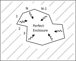
For a perfect enclosure, the row sum must satisfy the following requirement:


where Fij are the view factor matrix values.
For a leaky enclosure, the row sum must satisfy the following requirement:


For a perfect enclosure, the following residual must be less than the specified convergence value (input as CONV on the VFSM command).

where ' indicates the new view factor values.

For a leaky enclosure, the following residual must be less than the specified convergence value (input as CONV on the VFSM command).

where Fij is the original view factor values.

To ensure a good energy balance, the following reciprocity relationship must also be met:

where Ai is the area of the ith facet.

View Factor Matrix: General
For a perfect enclosure with N facets, the view factor matrix is:
 | (6–16) |
where:
Fij represents the fraction of radiation energy leaving facet i and hitting facet j.
Consequently, the following requirements must be satisfied:
summation:  for all i = 1,2, … N
reciprocity:  for all i and j, where
Ai
is the area of facet i.
for all i and j, where
Ai
is the area of facet i.
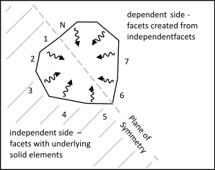
View Factor Matrix for a Model with Symmetry
For a model with symmetry defined by issuing the RSYMM command, we can decompose the view factor matrix as:
 | (6–17) |
where the subscripts,  and
and  , denote independent and dependent. Independent facets have underlying solid
elements underneath while dependent facets are created from independent facets using
RSYMM settings, as illustrated in Figure 6.6: View Factor Facets for a Model with Symmetry.
, denote independent and dependent. Independent facets have underlying solid
elements underneath while dependent facets are created from independent facets using
RSYMM settings, as illustrated in Figure 6.6: View Factor Facets for a Model with Symmetry.
The reciprocity condition is written as:
 | (6–18) |
where:  .
.
Here,  and
and  represent a block diagonal matrix of the independent and dependent facet
areas, respectively.
represent a block diagonal matrix of the independent and dependent facet
areas, respectively.
Based on symmetry:
 | (6–19) |
Substituting Equation 6–19 and Equation 6–17 into Equation 6–18 and simplifying gives:
 | (6–20) |
(When numerical methods are used, Equation 6–20 is approximate.)
This means  matrix is symmetric,
  .
.
Also note that block lumping gives
 | (6–21) |
where  .
.
When condensed view factor is turned on (VFCO is issued with
LEVEL=1 or 2), the view factor matrix produced is  .
.
When condensed view factor is turned off (VFCO command is not used
(default) or is issued with LEVEL = 0), it is  .
.
Four methods for analysis of radiation problems are included:
Radiation link element LINK31(LINK31 - Radiation Link). For simple problems involving radiation between two points or several pairs of points. The effective radiating surface area, the form factor and emissivity can be specified as real constants for each radiating point.
Surface effect elements - SURF151 in 2D and SURF152 in 3D for radiating between a surface and a point (SURF151 - 2D Thermal Surface Effect and SURF152 - 3D Thermal Surface Effect ). The form factor between a surface and the point can be specified as a real constant or can be calculated from the basic element orientation and the extra node location.
Radiation matrix method (Radiation Matrix Method). For more generalized radiation problems involving two or more surfaces. The method involves generating a matrix of view factors between radiating surfaces and using the matrix as a superelement in the thermal analysis.
Radiosity solver method (Radiosity Solution Method). For generalized problems in 3D involving two or more surfaces. The method involves calculating the view factor for the flagged radiating surfaces using the hemicube method and then solving the radiosity matrix coupled with the conduction problem.
A mass transport option is available for the current-technology elements, SOLID278 and PLANE292, and the legacy elements, PLANE55 and SOLID70, to simulate the mass transport of heat by a flow with a prescribed velocity field in your analysis. The option to include mass transport is controlled by KEYOPT (8) for PLANE55, SOLID70, and PLANE292 and KEYOPT(11) for SOLID278. This section discusses the governing equations and restrictions for mass transport simulation. For procedural details and information on setting up an analysis to simulate mass transport and example problems, see Mass Transport (Advection) in the Thermal Analysis Guide.
Figure 6.7: Mass Transport Problem in a Flow Field shows the directed flow field (orange arrows) over a domain
 with a surface
  and the unit vector
  normal to its surface. The surface can be split into the inflow side
 where
where  and the outflow side
  where
where  , and
, and 
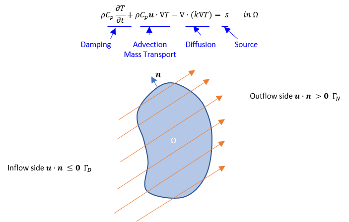
The equation in Figure 6.7: Mass Transport Problem in a Flow Field is the first law of thermodynamics in differential form (Equation 6–1 rewritten), and the second term describes mass transport. Typically, the Dirichlet boundary condition is applied on the inflow side and the Neumann boundary condition is applied on the outflow side as follows:
Dirichlet boundary condition: 
|
Neumann boundary condition: 
|
These are the only boundary condition options available for legacy elements PLANE55 and SOLID70.
For current-technology elements PLANE292 and SOLID278, you can choose between two types of Neumann boundary conditions described below.
The diffusive flux (Dflux) formulation is, again, the same as that for PLANE55 and SOLID70:
Neumann boundary condition: 
You specify the Dflux Neumann boundary condition by setting KEYOPT(8) =1 for PLANE292 and KEYOPT(11) =1 for SOLID278. The total flux (Tflux) formulation includes the advective term in the Neumann boundary condition as follows:
Neumann boundary condition: 
You specify this Tflux Neumann boundary condition by setting KEYOPT(8) = 2 for PLANE292 and KEYOPT(11) = 2 for SOLID278.
There are pros and cons associated with either of these boundary conditions. The main advantage of the Tflux formulation is that it will satisfy an energy balance with the PRRSOL command, but setting up its Neumann boundary condition is slightly more complex since it includes both a diffusive and an advective flux. Vice versa, if you are not interested in the energy balance, you could use the Dflux boundary condition which is easy to set up.
Imposing the Neumann Boundary Condition
Specifying a known heat flux
To specify a heat flux at the outlet as the Neumann boundary condition, issue the
SF or SFE command with Lab =
HFLUX and specify its value. Specifying a known heat flux Neumann boundary condition is the
same for both the Dflux and the Tflux formulation.
Specifying zero diffusion flux for high Peclet number
Since the diffusion flux becomes negligible at high flow rate, it is typical for high Pe
to specify a soft boundary condition of zero diffusion flux on the outflow side,
 .
.
- Dflux formulation
This is easily accomplished with the Dfulx formulation of the Neumann boundary condition. To set
 on the boundary, no commands are required since the default value of
Lab= HFLUX (on SF or SFE) is zero.- Tflux formulation
It is less straightforward to specify zero diffusion flux on the outflow side under the Tflux formulation. Setting
 , the Tflux Neumann boundary condition becomes
  , which you can set as a convection boundary condition. To do so, issue
the SF or SFE command with
, which you can set as a convection boundary condition. To do so, issue
the SF or SFE command with
Lab= CONV, and specify the bulk temperature = 0 and the known value of the film coefficient to .
.