


Topics in this section:
The Imported Solid Model feature enables you to map the Composite Definitions of ACP (Pre) onto the mesh of an external (imported) solid model. This approach can be used if the standard solid model approach, that is based on an extrusion algorithm and post operations, fails or produces a mesh of poor quality. In that case, it is more robust to mesh the final composite solid structure first, independent of the lay-up data and, in a second step, to map the Composite Definitions. See the Guide to Solid Modeling section for solid model workflows as well as tips used when working with a solid model.
The Imported Solid Model (containing lay-up mapping data) can be used in combination with structured elements (such as brick, prism, or wedge) and degenerated shapes (tetra and pyramid). The Lay-Up Mapping Objects feature provides several options to control the mapping. For more information on the element technologies, material handling, and element orientations, see Lay-up Mapping Objects. The imported solid mesh with the mapped lay-up data is exported for downstream analyses using the standard solid model workflow in Workbench.
The lay-up mapping feature is the 3D representation of the lay-up model computed immediately after the imported solid model updates. This 3D representation always follows the surface normal of the shell mesh. The imported solid model does not support the Extrusion Guides feature. If you need to manage the free edges in curved areas, one recommended approach is to enlarge the shell surface and plies in the in-plane direction.
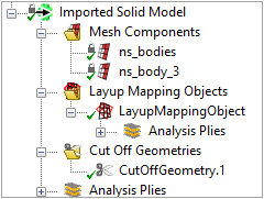
The elemental component sets that are defined in the external solid mesh are listed in the Mesh Components sub-folder and are used to define the scoping of the Lay-up Mapping Objects. All component sets (also node sets) of the initial solid mesh are passed as Named Selections to the downstream analyses (Mechanical Model) and can be used to maintain correct associations (such as boundary conditions or contacts).
See the Analysis of a Mapped Composite Solid Model section for an example analysis.
Cut-Off Geometries can be used to shape the Imported Solid Model in a desired way. They are specified in the respective subfolders in the Imported Solid Model Tree View. The Cut-Off feature behaves in the same way for the Imported Solid Model as it does for the standard Solid Model. It is described in Cut-Off Geometry. The Analysis Plies sub-folder shows which Analysis Plies are incorporated in the lay-up mapping.
This Cut-Off feature allows you to shape the imported solid mesh after the lay-up mapping. It gives you further control of geometry and mesh. You can add details and geometrical features to the Imported Solid Model. Therefore, the generation of a structured mesh will be easier and more robust for many cases.
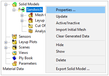
The context menu of the Imported Solid Model contains these actions:
Properties: Opens the Properties dialog of the imported solid model.
Update: Runs the lay-up mapping algorithm and updates all dependencies of the Imported Solid Model.
Active/Inactive: Toggle whether the Imported Solid Model is suppressed or not.
Import Initial Mesh: Loads the initial mesh of the solid model without performing the lay-up mapping.
Clear Generated Data: Removes all elements and mapped lay-up data from the object.
Hide: Hide the solid model in the Scene.
Show: Show the solid model in the Scene.
Delete: Delete the Imported Solid Model. Not possible if the object is locked.
Export Solid Model: Export the mesh or skin of the solid model as a geometry or as a Mechanical APDL input file.
You can configure the settings for the Imported Solid Model under the Imported Solid Model context menu item Properties. The properties dialog covers some basic settings where the scope of the lay-up mapping is configured through the Lay-up Mapping Objects.
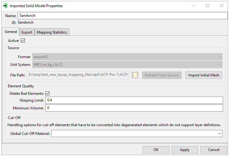
Name: Name of the object
Format: This property specifies the format of the input file. Within a Workbench project, solid meshes are imported via a Mechanical Model component. The import automatically completes the Format, Unit System, and File Path properties, so as a result, these properties are read-only.
If you are running ACP in standalone, you can directly import Ansys CDB files in ACP Pre. For this scenario, you need to specify the Unit System of the volume mesh.
Unit System: This property specifies the unit system of the external solid mesh which is used to automatically convert the solid mesh into the unit system of ACP.
File Path: Specifies the location of the mesh file to be imported.
Refresh From Source: Only enabled in ACP standalone. Click to prompt ACP to reread the mesh from the source file. Use this feature whenever the source file is modified because ACP does not re-read the data automatically.
Import Initial Mesh: Loads the initial mesh of the solid model into the ACP Model without performing the lay-up mapping. This can be used, for example, after using the Clear Generated Data feature, to show the initial mesh once again.
Element Quality (Delete Bad Elements, Warping Limit, Minimum Volume): See the explanation for Element Quality under Solid Model Properties.
Global Cut-Off Material: Controls the global material handling for Cut-Off Elements in the solid model. Cut-Off Elements which have a degenerated shape (tetra) do not support layers and therefore are filled with a Cut-Off material. This setting is used when the material handling settings for fabrics and stackups are set to Global. See Fabric Solid Model Options.
The export tab options are a limited set of the standard solid model options. See Export in the Solid Model Properties section.
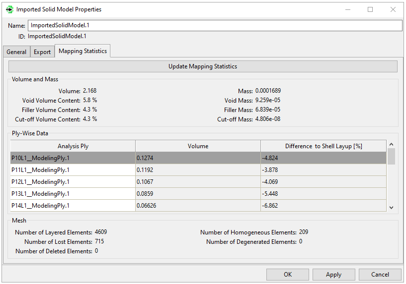
The Mapping Statistics tab includes basic results regarding the lay-up mapping such as total mass, volume, resin volume content, and so on. The Ply-Wise Data table shows the volume per analysis ply and the difference compared to the lay-up definition based on the shell mesh. The solid mesh ply volume is greater if the difference is positive, smaller if negative.
Mesh Components (Element Sets) in the external solid mesh are listed in this folder. Mesh Components are either:
Named Selections in Mechanical
Component sets in Mechanical APDL
Or components of elements in the external mesh generated by a third-party meshing application
Note that Mesh Components cannot be visualized in the Scene until the initial mesh is loaded. This happens when you Import Initial Mesh or Update the Imported Solid Model. Mesh Components cannot be edited nor copied, and they are read-only.
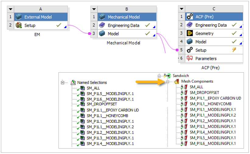
Figure 2.149: Transfer of Mesh Components from an External Mesh via External Model, Mechanical to ACP Pre
This folder contains the Lay-up Mapping Objects used to define mapping scopes and to configure material handling. An Imported Solid Model can have multiple Lay-up Mapping Objects defining which plies are mapped to which components of the solid mesh. Note that the node connectivity remains unchanged, regardless of the number of Lay-up Mapping Objects.
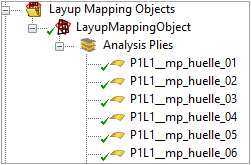
The Analysis Plies folder under a Lay-Up Mapping Object lists all the imported and/or simple Analysis Plies of the source scope. The list becomes available after updating the object and helps to verify the source scope.
The properties of the Lay-up Mapping Object are split into General, Layered Elements, and Reinforcing.
The General tab configures the source and target scopes of the lay-up mapping. The source scope is defined by a set of shell elements and a list of plies. The mesh components of the solid mesh define the target scope. This enables a component-wise mapping of the lay-up model onto the solid mesh.
The Element technology for Imported Solid Models is the lay-up mapping feature that supports layered and reinforcing elements. You can configure it in the General tab or the respective option's tab. The following contains more information on the two Element technology options:
Layered Elements
The layered element technology should only be used if the solid mesh consists mainly of brick or prism elements, which are then treated as layered ones. These elements are automatically aligned according to the normal direction of the lay-up and are filled with layers.
Note: If the layered element faces are not parallel to the lay-up direction, there might be inaccuracy since its normal direction would differ from the lay-up direction.
Degenerated elements (pyramid, tetra, etc.) are filled with the filler material and become homogeneous elements, as well, because they do not support layered data. The element coordinate system of homogeneous elements can be defined by one or several rosettes.
Elements that do not intersect with the mapped lay-up can be deleted or filled with a filler material. In that case, they are handled as homogeneous elements.
Reinforcing Elements
The reinforcing element technology adds material to an existing element by intersecting the element with basic shapes (link, shell, etc.). For more information, see Reinforcing Elements in the Element Reference. This technology uses the REINF265 element which enables adding material to a 3D solid element. Therefore, it can be used with any solid mesh type. The solid elements are always homogenous, and their coordinate system is also defined by rosettes. Also, the reinforcing plies and their material direction are independent of the base element.
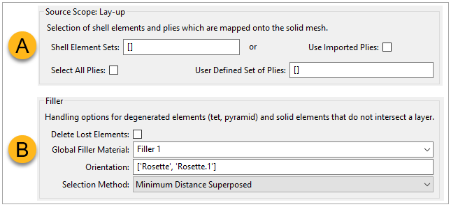
The Source Scope is defined by a set of shell elements and a list of plies, while the Target Scope is defined by the mesh components of the solid mesh. This enables a component-wise mapping of the lay-up model onto the solid mesh.
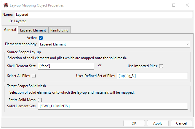
Source Scope: Lay-up
Shell Element Sets: Select one or several Element Set(s) to define the region of interest. Starting with a shell model and the lay-up definition, the 3D representation of the laminate is generated for the selected region.
Note: The Middle Offset option for Element Sets is not supported. The ply definition must be defined without this option to obtain an accurate mapping.
Use Imported Plies: If enabled, Imported Plies are mapped onto the solid mesh instead of the standard Modeling Plies. In this situation, the Shell Element Sets option becomes irrelevant.
Select All Plies: By default, this property maps all plies of the selected shell mesh (Shell Element Sets) onto the solid mesh. Clear this box to select a user-defined set of plies for the mapping. Modeling Groups and/or Modeling Plies can be selected.
If Use Imported Plies and Select All Plies are both enabled, all Imported Plies are selected.
User Defined Set: This field allows you to specify a set of Modeling Plies and/or Modeling Groups when selecting the plies to be mapped onto the solid mesh. The equivalent object types can be selected if Use Imported Plies is enabled.
Target Scope: Solid Mesh
Entire Solid Mesh: If selected, the source scope (lay-up) and materials are applied to the entire solid mesh. This also means that no other Lay-up Mapping Object can be configured because the Target Scope cannot overlap.
Solid Element Sets: Use this field to select the specific Mesh Components of the solid mesh to which the Lay-up Mapping Object will be applied. Mesh Components are Named Selections or Element Sets which are defined in the initial (external) solid mesh.
In most cases, the lay-up does not fill the entire selected target scope (solid elements), or there are voids (gaps between layers). Use the options in the Layered Element tab to configure how voids are handled as well as the lost elements which do not intersect with the lay-up. Because these layered elements are defined per Lay-up Mapping Object, an Imported Solid Model can have multiple void and filler materials.
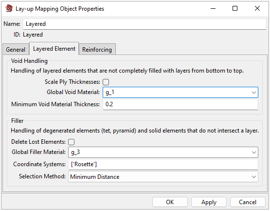
Void Handling
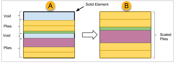
Scale Ply Thicknesses: The thickness of the mapped lay-up and the geometrical thickness of layered elements can differ for various reasons (drop-offs, numerical differences, and so on). If this option is enabled, the thickness of the mapped laminate will be scaled to match the element as shown below. Note that the scaling is done per element and not on a global scope. Below is a side view of a layered solid with void space (A) and the same element after the ply thickness has been scaled (B).
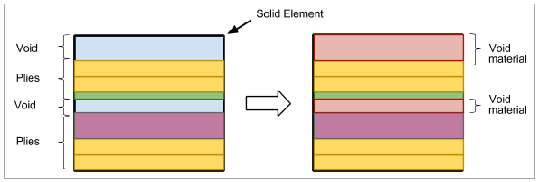
Global Void Material: Instead of scaling the laminate, you can fill the void space with a specific material. To do so, be sure to clear the option Scale Plies and then define a void material. Use an isotropic material since the in-plane orientation cannot be defined.
Note that you can access elements with void material through the analysis ply void_<material id> within the Analysis Plies folder of the Imported Solid Model. There are as many void layers in the folder as the maximum number of void layers in a layered element. For instance, in the illustration below, there are two void spaces in a layered solid element.
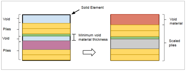
Minimum Void Material Thickness: Void spaces, like those shown above, can be caused by drop-offs or differences between the shell and solid mesh, especially in curved areas– to name some examples. You can further refine the void handling by specifying the Minimum Void Material Thickness. If the thickness of the void space is less than the specified value, the void will not be filled. Instead, the regular plies are scaled to fill the void space.
In the illustration below, scaled layers and filled void space are both applied.
This raises a possible point of confusion: Why does ACP scale the plies if the option Scale Plies has been disabled? The fact is, the solver automatically scales the laminate whenever the total laminate thickness does not correspond with the element height, so ACP is performing the scaling already. The Minimum Void Material Thickness feature allows you to visualize and express numerically this effect in ACP.
Filler
Elements which do not intersect with the lay-up are called lost elements. They are either deleted or filled and oriented with a Filler Material and Rosette(s), respectively.
Delete Lost Elements: Use this option to control whether solid elements without mapped lay-up data are removed or retained. Note that unstructured elements such as tets or pyramids are ignored in the mapping algorithm and are always treated as lost elements (elements without data).
Global Filler Material: If the property Delete Lost Elements is disabled, a filler material must be assigned to the solid elements that do not have mapped lay-up data. Lost elements are handled as non-layered (homogeneous) elements. The characteristic of the filler material can be isotropic or anisotropic.
Note: The homogeneous elements with filler material can be accessed through the analysis ply filler_<material id> within the Analysis Plies folder of the Imported Solid Model.
Orientation: Select one or several Rosettes to orient the filled elements. Note that the Rosettes are used to evaluate the fiber directions (local x-axis) and the normal directions (local z-axis) of the elements. This is slightly different compared to Oriented Selection Sets where the Rosettes are used to apply the reference directions only.
If the Normals and Fiber Directions plot is enabled, you can visualize the element's x and z axes by selecting the filler layer.
Selection Method: Supported options include Minimum Distance and Minimum Distance Superposed as described in Oriented Selection Set.
Use Filler Option Only: The Lay-Up Mapping Object also allows you to fill Mesh Components or the entire solid mesh with a filler material and to orient the elements so that no plies from the lay-up are mapped. To do so, define an empty Source Scope in the General tab (A, below). In the Materials tab (B), clear the Delete Lost Elements option, and select a Filler Material and Rosettes.
The mapping algorithm, based on the 3D representation of the lay-up, consists of three main steps:
Aligns the structured solid elements according to the local offset direction of the 3D representation.
Evaluates the ply-wise intersections between the solid elements and plies. The mapping algorithm also detects if an element is completely within a ply. The output contains the element-wise plies' materials, thicknesses, and orientations. Thus, the element-wise section data.
Stores the data for downstream analyses.
Note: The mapping algorithm evaluates the intersection at the center of the solid elements, therefore, the ply thicknesses are constant for the whole element.
The following limitations are specific to the layered element technology:
The projection of the failure results to the reference surface is not supported. Either do ply-wise analyses or use the Section Cut feature in Mechanical to investigate results inside the solid.
Laminate failure criteria such as Wrinkling and Shear Crimping are not supported since the reconstruction of the stacking sequence of the laminate is not possible for mapped lay-up data.
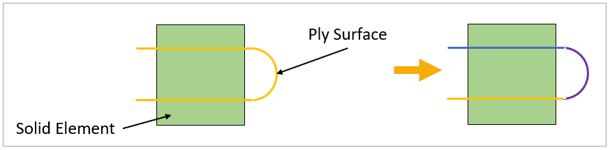
The mapping algorithm assumes that an analysis ply intersects only once with a solid element. Therefore, the scenario on the left side of the image is not supported, and the generated data is incorrect. A workaround is to split the ply as shown on the right side.
This tab becomes active when the Element technology is set to reinforcing. It enables the control of reinforcing elements' section properties and the configuration of the 3D solid elements' material and orientation.
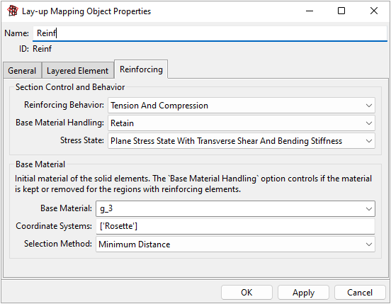
Use the following options to configure the reinforcing elements' structural behavior. For more information, see SECCONTROL:
Reinforcing Behavior: Specifies whether the reinforcing elements carry tension and compression load, or only one of them.
Base Material Handling: Removes the base material from the solid element where it intersects with the reinforcing elements or, otherwise, retains the base material. It is recommended to select remove if a high-volume fraction of reinforcing elements is expected.
Stress State: Specifies if the reinforcing elements should behave like a link, membrane, or shell element (with or without bending). For more information, refer to SECCONTROL– Type: REINF.
Reinforcing elements use the stiffness of the plies for the solid elements. An initial material must be assigned to the solid elements because it is possible that some elements are not reinforced. The following options enable the specification of the initial material and orientation (if the material is orthotropic):
Base Material: Specifies the solid elements' material before the reinforcing elements are applied. The base material characteristic can be either isotropic or anisotropic.
Orientation: Selects one or more rosettes to orient the solid elements. Here, rosettes are used to evaluate the material 1 directions (local x-axis) and normal directions (local z-axis) of the elements. These characteristics are different from Oriented Selection Sets (OSS), where the rosettes are only used to apply the reference direction.
Selection Method: Supported options are Minimum Distance and Minimum Distance Superposed as described in Oriented Selection Sets (OSS).
Mesh Quality
You can use the reinforcing technology with all solid element types (brick, prism, pyramid, or tetra). Nevertheless, their shape must be of good quality, and not too distorted, so the reinforcing elements can successfully apply to the base elements.
Element Size vs Ply Thickness
You can independently define the reinforcing elements of the base elements, including their size, shape, and element formation. It is essential that the plies' thickness is smaller than the base elements' size. This ensures that the reinforcing elements' stiffness accurately applies to the base elements. For instance, you can model thick plies, such as core materials, with multiple thin plies instead of one thick ply. For more information, see Number of Layers in Modeling Ply Properties.
Cut-Off Geometry
You can use the Cut-Off Geometry feature with the reinforcing elements. The algorithm might result in solid elements with reduced shape quality and cause issues when combining the reinforcing elements with the base elements. Therefore, you should mesh the final geometry instead of shaping the solid mesh in ACP with cut-off geometries.
The following limitations are specific to the reinforcing element technology:
The standard composite post-processing features (failure tool, ply-wise result visualization, etc.) are not supported for reinforcing elements. Use Mechanical APDL for post-processing your analysis.
The composite workflows in Workbench does not support reinforcing elements and will skip all of their instances. The complete solid model with reinforcing elements can be exported to Mechanical APDL via Export Solid Model from the context menu of the Imported Solid Model.
The analysis ply thickness should be smaller than the solid elements' height. Otherwise, the contribution of the reinforcing elements to the element stiffness might be incorrect. For more information, see Design Tips and Best Practices.
The application offers several options to verify the quality of the mapped lay-up.
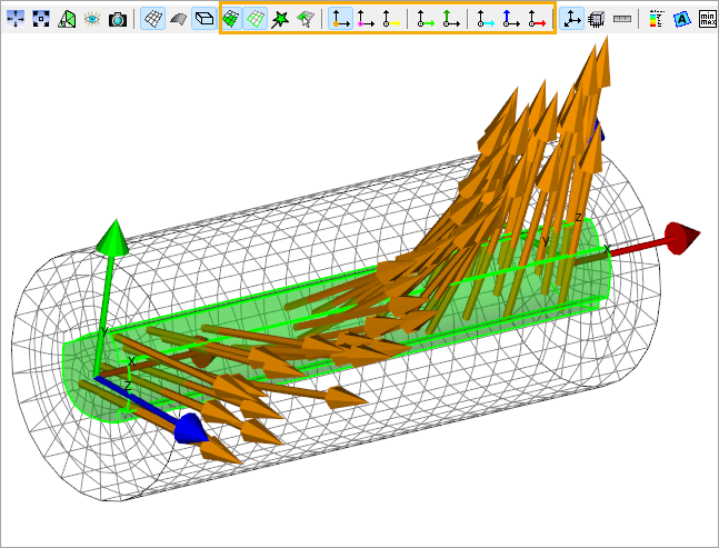
You can examine the fiber directions and element normals using the Orientation Visualizations options on the Toolbar.
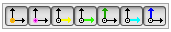
Make sure that the solid elements are highlighted by having these mesh appearance settings:
 or
or 
You can use the Thickness Plot to display the ply-wise thicknesses on the solid elements. You can also select the Component option to plot the ply-wise scaling factors.
lay-up Mapping Plot enables you to plot ply-wise volume contents and the deviation of the normal direction between the shell mesh and solid mesh. This plot works only if the Element technology is set to layered elements.
You can get a general overview using the mapping statistics if the Element technology is set to layered elements.
Reinforcing Elements: A model that can also be reviewed in Mechanical APDL. These Mechanical APDL commands show the reinforcing elements together with the reinforced solid elements.
alls
esel,u,ename,,REINF265
/trlcy,elem,0.9
esel,all
! Enable the expanded element shapes.
/eshape,0.05
eplot
The following commands are used to plot the main material (reinforcing) direction.
/dev,vect,1
! Select only reinforcing elements (optional)
esel,s,ename,,REINF265
/psymb,layr,-1
eplot
The global model property 'minimum analysis ply thickness' also counts for the lay-up mapping. A layer is only added to an element if the mapped layer thickness is greater than this value.
The lay-up representation (shell) is ignorant to the concept of Drop-Off elements (solid) and this can lead to 'voids' if you have steps in the lay-up as shown in the figure below. If the drops are low, this can be neglected, if they are high you might have to refine the tapering or adjust the void handling of the imported solid model.

In general, the mapping is mesh independent and the shell and solid mesh do not have to be coincident. However, too big of a difference in the meshes might cause inaccurate results. Therefore you should work with meshes with similar element sizes, especially in curved regions.
The shape functions of the shell and solid elements can differ. For instance a Composite Definition of a linear shell mesh can be mapped onto a quadratic solid mesh.
Full cross-sections: The mapping might does not work as expected for plies that shrink into a very small tube as pictured below on the left hand side. In that case, it is more robust to have several plies of moderate thickness instead of one thick ply as shown by the right picture.
