


This section outlines the beta features supported by the Fluent GPU Solver. For information on defining settings for the beta features listed below, refer to their relevant sections in the Fluent User's Guide.
The following beta features are available when using the Fluent GPU Solver:
Surface to Surface (S2S) and Discrete Ordinates (DO) radiation models.
Note: The following limitations apply:
The S2S radiation model is not supported for mesh motion (dynamic meshes, sliding meshes, and wall motion) or periodic boundaries.
The WSGGM (weighted-sum-of-gray-gases model) is not supported for the GPU implementation of the DO model (gives incorrect results).
Anisotropic thermal conductivity. See Anisotropic Thermal Conductivity for Solids in the Fluent User's Guide for details.
Optimized LES Numerics. See Optimized LES Numerics for details.
Viscous heating effects for turbulence modeling. See Including the Viscous Heating Effects for details.
Curvature Correction for turbulence modeling.
Algebraic Transition model for turbulence modeling.
Standard Roughness Model with constant parameters per wall boundary.
Adiabatic FGM combustion model. See Flamelet Generated Manifold for details.
Poor mesh numerics can be enabled by entering the following command in the console:
/solve/set/poor-mesh-robustness/poor-mesh-numerics
						yes
Ffowcs Williams and Hawkings Acoustics Model including FFT of surface pressure fields. See Ffowcs Williams and Hawkings Acoustics GPU Model for details.
The Fluent GPU Solver supports the reading of settings only case files as outlined in Reading Settings Only for Mesh or Case Files with Large Cell Counts in the Fluent User's Guide. This allows for cases with large cell counts to be quickly and efficiently modified, then read into the GPU Solver for restarting a calculation.
Static expressions.
User-defined scalar (UDS) equations. See User-Defined Scalar (UDS) Transport Equations in the Fluent User's Guide for details.
Transient profiles.
EnSight DVS files for exporting solution data. For details, see Exporting Solution Data as EnSight DVS Files.
Restarting the Fluent GPU Solver calculation in such a way as to minimize the needed CPU resources. For details, see Restarting a Calculation with Minimal CPU Resources.
Discrete Phase Model (DPM). For details, see Discrete Phase Model (DPM) .
User-defined functions (UDFs) written in Python, which can make use of the massively parallel computations enabled by the Native GPU Solver. For details, see Python User-Defined Functions (UDFs). Note that the traditional UDFs written in C have limited support (as described in C User-Defined Functions (UDFs) with the Fluent GPU Solver), and only a subset of their functionality works with the GPU solver.
GPU/CPU remapping.
GPU/CPU remapping is available as a beta feature for handling tasks across multiple CPU and GPU resources and can lead to potential performance gains. The use of GPU/CPU remapping is particularly useful in optimizing computational tasks that are GPU-intensive, ensuring that GPUs are utilized as efficiently as possible, based on specific workload needs and system architecture.
Note: GPU/CPU remapping is not supported when using Discrete Phase
Model (DPM) or Acoustics models. If DPM or Acoustics models
are enabled before or during the simulation after activating
-gpu_remap, the Fluent
GPU solver will revert to one-to-one GPU/CPU mapping.
Default remapping can be specified by adding either the
-gpu_remap or
-gpu_remap=1 command when launching
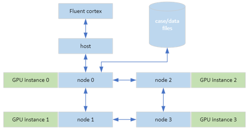
the GPU solver from the command line as outlined in Starting the Fluent GPU Solver from the Command Line. For default remapping, all CPU
partitions are merged evenly and the computational workload is
distributed to all available GPUs across all machines in the network
or cluster as shown in Figure 33.1: Default Remapping.
This approach is aimed at maximizing the utilization of GPU
resources across different hardware, enhancing overall computational
efficiency.
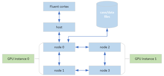
Alternatively, -gpu_remap=2 can be entered to
change the default remapping behavior and assigns all CPU partitions
to processes that exclusively utilize the GPUs within the same
machine as shown in Figure 33.2: 2 to 1 Remapping. This
approach could be beneficial in scenarios where minimizing data
transfer between machines can lead to better performance due to
reduced network overhead or latency.
User-defined scalar (UDS) transport equations are supported by the Fluent GPU Solver as a beta feature, with the following general limitations:
Up to 50 transport equations can be defined and solved.
UDS equations can only be used for fluid zones.
Only single phase flow is supported.
Convective flux can be set as On or Off (UDF is not supported).
Inlet diffusion can be set as On or Off.
Source Terms can be defined as constant or using a profile or expression.
The Unsteady Function must be set to default.
The UDS Diffusivity must be constant.
Solution setup •Discretization scheme (per-uds) and relaxation parameters (common)
In the Solution Controls task page, the discretization scheme must be defined as per-uds with default relaxation parameters.
The Fluent GPU Solver supports the use of transient profiles to define boundary and cell zone conditions as a beta feature, with the following general limitations:
Transient periodic profiles are not supported.
Only piecewise linear interpolation is supported.
When using a transient profile with a steady state simulation, the initial condition of the profile (t=0) will be used.
Cell zone condition Source Terms can be defined using transient profiles for energy and momentum with the following limitations:
All three components of momentum must be of type transient profile.
More than one transient profile per equation can not be used.
Constant values can be specified for parameters in combination with transient profiles.
Steady profiles can not be used in combination with transient profiles.
The following limitations apply to setting up boundary conditions using transient profiles:
Transient profiles can be used for the following settings under the Momentum and Thermal tabs, for all types of boundary conditions:
For Momentum options,
Static pressure
Temperature
Mass flow rate
Velocity can be specified as Magnitude and normal, Components, and Magnitude and direction (direction can not be specified as transient profile; only the magnitude can vary with time)
For Thermal options,
Heat flux
Heat generation rate
Temperature
Free stream temperature
Heat transfer coefficient
Radiation temperature
Emissivity
An optimized LES numerics scheme in available for the GPU solver. The optimized scheme typically allows for a reduction in the number of iterations used per time step (two iterations are often sufficient). In the case of continuity residuals not dropping for the second iteration, reducing the time step size provides better accuracy improvements over increasing the number of iterations per time step used, and eventually leads to better continuity residual behavior.
From the Viscous Model dialog box, when Large Eddy Simulation (LES) is selected, Optimized LES Numerics is available under LES Model Options.
Upon activation, the following TUI commands are enabled:
/solve/set/enhanced-les-numerics/optimized-advection? yes 1.0 0
Uses the approximate 4th order reconstruction scheme for advected quantities.
/solve/set/enhanced-les-numerics/optimized-cd? yes
Changes pressure-velocity coupling and pressure discretization.
/solve/set/enhanced-les-numerics/optimized-algorithm? Yes
Sets momentum and pressure under-relaxation factors to 1. Sets use of SIMPLEC. Sets pressure-skew corrections to 0
Notes:
The changed advection scheme is not shown in the discretization panel, but only noted in the transcript.
Only for use with second order time discretization (default for LES).
This method can typically (tested mostly on high quality meshes) run without under-relaxation factors (1.0). In case of robustness issues, try setting momentum under-relaxation to 0.7.
The integral aeroacoustics model by Ffowcs Williams and Hawkings (FW-H) and its usage in Ansys Fluent are described in The Ffowcs Williams and Hawkings Model in the Fluent Theory Guide and Using the Ffowcs Williams and Hawkings Acoustics Model in the Fluent User's Guide. With Ansys Fluent 2024R1, you can use this model with the Fluent Native GPU solver.
This is done using the two step acoustics calculation workflow as follows:
Export the sound source data to a file during a transient flow simulation.
Import of the exported data to compute the sound signals, after simulation is finished.
This workflow is equivalent to the CPU solver, however the file format for the sound
source data has the extension .asdg (instead of
.asd for the CPU solver), and data from each mesh partition are
exported to a separate file using a parallel output method. This is done to accelerate the
output process and prevent a performance slowdown when using the fast GPU flow
solver.
Because the file format is different, it is not possible to continue a CPU-written
source data export in a FluentGPU session. If you load an existing FW-H setup, which was
created using the Fluent CPU solver, to a Fluent GPU session, you will have to ensure
that the index file does not contain lines with the .asd extension.
The recommended workflow in this case is to revisit the FW-H model (using GUI or TUI) in the
GPU session and click in both the Acoustic
Sources and Acoustic Model dialog boxes (or click through
the corresponding text commands). This will re-create the index file and the model-specific
solver settings. There is no need to revisit the receivers' specification.
The following limitations apply to the FW-H model in Fluent 2024R1:
Only the two-step acoustics calculation mode is available. The on-the-fly calculation of sound signals during the transient flow simulation is not supported.
Grid partitioning cannot be changed during the data export and the sound signals’ computation. After the desired partitioning for the flow simulation is created, the case file must be written to a disk and re-read back in Fluent in the same or in a following session before beginning with the FW-H source data export.
This is necessary to establish the final ordering of mesh element faces.
The use of the FW-H model with a steady-state simulation of a rotor in a rotating reference frame is not supported.
The exported
.asdgfiles can be used for FFT of the static pressure transient fields. When using this feature in a separate Fluent GPU Solver session, the grid partitioning must be kept the same as that used in the data export session.
When using the Fluent GPU Solver, the exporting of solution data as EnSight DVS files has beta support. Note the following differences when exporting such files when the data was calculated by the GPU solver compared to that generated by the CPU-based solver (as described in EnSight DVS in the Fluent User's Guide):
Exporting should be faster.
You are able to specify that data is exported from both cell zones and surfaces, not just one or the other.
You cannot export data from the nodes, only the cell centers.
To export solution data after a steady or transient calculation by the Fluent GPU Solver, perform one of the following:
Use the File/Export/Solution Data... ribbon tab option to open the Export dialog box, select EnSight DVS from the File Type drop-down list, and make selections from the Cell Zones and/or Surfaces lists, as well as the Quantities list. Then click the button and specify the name of the file in the Select File dialog box that opens.
Use the following text command:
file→export→ensight-dvs
To export solution data during a transient calculation by the Fluent GPU Solver, perform one of the following prior to running the calculation:
Use the File/Export/During Calculation/Solution Data... ribbon tab option to open the Automatic Export dialog box, select EnSight DVS from the File Type drop-down list, and make selections from the Cell Zones and/or Surfaces lists, as well as the Quantities list. Then make selections from the Export Data Every drop-down lists, enter a File Name, and click the button.
Use the following text command:
file→transient-export→ensight-dvs
The Fluent GPU Solver typically utilizes both GPU and CPU resources. The ability to restart the calculation in such a way as to minimize the needed CPU resources is supported as a beta feature. To do such a restart, perform the following steps:
Launch a session of Fluent in one of the following ways, so that you can create the restart files:
Launch the Fluent GPU Solver in the typical fashion (that is, using the
-gpucommand line option or by enabling the Native GPU Solver option in Fluent Launcher).Launch Fluent on a machine without any GPUs, using the
-gpu=-1command line option.
Then perform the following:
Create a 3D case and data file pair (for details, see Using the Fluent Native GPU Solver in the Fluent User's Guide).
Note: You must ensure that you write the resulting files in the Common Fluids Format (with the
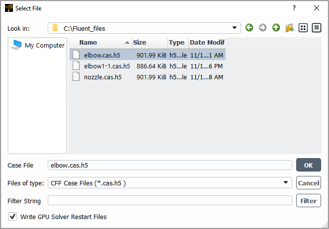
.cas.h5and.dat.h5extensions).Write restart files by performing one of the following:
Open the Select File dialog box by clicking either the File/Write/Case... or File/Write/Case & Data... ribbon tab item; then enable the Write GPU Solver Restart Files option, enter a Case Name, and click .
Use the following text command:
file→write-gpu-restartNote that a folder will be created that uses your case file name as a prefix, and that contains
.pcasand.restartfiles.
Continue the calculation:
Launch an appropriate version of Fluent and read your case file by performing one of the following:
Launch a new session of the Fluent GPU Solver from the command line or Command Prompt window, adding a
-liteoption to specify the use of a version that is designed for dealing exclusively with lightweight settings. Note that you must ensure that you specify the same precision as the session used in the previous steps; for example, if you previously used double-precision, the full command would befluent 3ddp -gpu -lite. Then read the case file you created in the original Fluent session.Launch a new session of the Fluent GPU Solver in the typical fashion (that is, using the
-gpucommand line option or by enabling the Native GPU Solver option in Fluent Launcher). Note that you must ensure that you specify the same precision as the session used in the previous steps. Then read the case settings only of the case file you created in the original Fluent session; for example, you could read it using the File/Read/Case Settings Only... ribbon tab item.
Review and/or modify the settings as necessary. For any operation that is related to the manipulation of the mesh, the graphical user interface (GUI) is grayed out, and the text command is unavailable; additionally, the
define/models/addon-moduletext command is unavailable.Run the calculation. Note that there is no need to initialize first, but you can if you would like to reset the data.
If you want to postprocess the results, perform one of the following:
As the calculation proceeds, export solution data as EnSight DVS files (as described in Exporting Solution Data as EnSight DVS Files) and view them using EnSight.
Write restart files, as described previously. Then launch either the Fluent GPU Solver (for example, using the
-gpucommand line option) or Fluent on a machine without any GPUs (using the-gpu=-1command line option), using the same precision used in previous steps. Next, read the case file you created in the original Fluent session. Finally, use thefile/read-gpu-restarttext command to read the most recently saved restart files and view the results.
When using the Fluent GPU Solver, the discrete phase model (DPM) is supported as a beta feature with the following capabilities and limitations:
Massless, inert, and droplet particle types can be tracked.
Both the steady and unsteady flow solvers are supported, but only transient particles are allowed.
The steady tracking scheme available with the CPU-based Fluent solver cannot be used with the GPU solver.
With the Fluent GPU solver, pathlines can be displayed for postprocessing however, the pathlines will be calculated using the CPU-based Fluent solver.
The default High-Res Tracking particle tracking option available with the CPU-based Fluent solver is used exclusively when using the Fluent GPU solver.
Barycentric interpolation is used to interpolate flow solver variables like velocity and turbulence quantities to the particle position.
By default, Fluent will use cell-center values of flow density and viscosity when calculating forces on the particle. If these properties vary with position, it is recommended that they are interpolated to the particle position as well. See Tracking Settings for the Discrete Phase Model for details.
The following DPM model injections can be used with the GPU solver:
Single injection
Surface injection
Group injection
Hollow-cone injection
Solid-cone injection
When the transient flow solver is used, particles will be injected at each flow timestep if the flow time is between the specified Start Time and Stop Time for the injection. Note that DPM parcels are created using the CPU-based Fluent solver, which are then uploaded to the GPU solver. Therefore, DPM parcels cannot be recomputed each time the particle solver is executed. Surface injections with the Randomize Starting Points option enabled will provide random initial positions but the starting positions will not change every time DPM parcels are injected.
When integrating the particle trajectory, physics is limited to drag and gravity/buoyancy for spherical particles. If gravity is enabled for the flow solver, gravity/buoyancy is automatically included in the calculations for the particle trajectory. If temperature is being solved in the continuous phase, then the particle temperature will also be solved. Convective heat transfer to and from the particles will be modeled using the Ranz-Marshal heat transfer coefficient. Evaporation and boiling can be modeled with the Convection/Diffusion-Controlled model for particles of type Droplet. Note that Pressure Dependent Boiling, Temperature Dependent Latent Heat, and Variable Lewis Number options are all enabled when using the GPU solver. To account for turbulent fluctuations, the Discrete Random Walk model with the Random Eddy Lifetime option is available. This model can only be enabled if turbulence modeling is enabled for the flow solver.
One-way particle-flow coupling is available in which the particle phase does not influence the continuous phase. Two-way particle-flow coupling can also be enabled by selecting the Interaction with Continuous Phase option in the Discrete Phase Model dialog box. Note that two-way coupling with mass transfer is not supported with the GPU Solver. When using two-way coupling, the Linearize Source Terms and Update DPM Sources Every Flow Iteration options are also available. Particle sub-cycling, in which particles are tracked multiple times within a single flow solver timestep, can also be used. This functionality is controlled by the DPM Iteration Interval entry in the Discrete Phase Model dialog box. For details on these settings, see Steady/Transient Treatment of Particles.
The SSD Breakup model is available when using the GPU Solver. This model can be enabled on the Discrete Phase Model panel and applies to all injections of type Inert or Droplet. Note that new child droplets are not spawned when using the GPU solver. Instead, breakup events lead to a decrease in the droplet diameter and a corresponding increase in the number-in-parcel to conserve parcel mass. The following SSD model parameters are hardcoded to the default values in Fluent:
Critical Weber Number = 6
Core B1 = 1.73
Xi = -0.1
Target Number In Parcel = 10
When using the Fluent GPU solver, the particle numerical methods cannot be modified. The trapezoidal Euler method will be used to calculate the particle position, while the implicit Euler method is used for particle velocity, temperature, and mass. Additionally, the accuracy control option available with the CPU-based Fluent solver is unavailable with the GPU solver. The particle integration timestep will be calculated from the Step Length Factor set in the Discrete Phase Model dialog box.
When defining boundary conditions for the Discrete Phase Model with the GPU solver, the Escape, Trap, and Reflect boundaries can be used. For wall zones, the default boundary condition is Reflect while boundaries associated with flow inlets and outlets will be Escape by default. It is also possible to sample particles at mesh face zones similar to when solving on the CPU-based fluent solver. However, sampling on postprocessing surfaces is not supported.
When using the Fluent GPU solver, the Graphical User Interface (GUI) will be restricted to DPM features that are supported. However, the Text User Interface (TUI) will not have such restrictions. As such, it is recommended that the GUI be used when setting up the DPM model to ensure that invalid options are not enabled.
Important: It is possible to enable unsupported features through the TUI. Doing so may result in a crash and total loss of data. Be certain that only supported features are enabled.
Note that when using the Fluent GPU solver, the DPM model is restricted to stationary meshes. Additionally, non-conformal interfaces are not supported. Zero-thickness walls (for example, baffles) should not be combined with the DPM model when using the Fluent GPU solver as the results will be inaccurate in the vicinity of the wall.
The Fluent Native GPU solver supports the use of user-defined functions (UDFs) written in Python as a beta feature, so that you can take advantage of the massively parallel computations. Your UDF code will largely retain the simplicity of the Python programming language, so that you can focus on the physical model. Internally, your Python code is transformed into machine code for use by the Native GPU Solver.
The following capabilities are supported:
profiles (for example, inlet velocity or temperature profiles)
source terms (for example, a temperature or momentum source over a cell zone)
properties (for example, changing the fluid flow viscosity to non-Newtonian or temperature-dependent viscosity)
To use Python UDFs with the Fluent Native GPU solver, perform the following steps:
Write a Python UDF file (for details, see the examples that follow), and save it in the same directory as the case file.
Hook the Python UDF by entering the following Scheme command in the console or the journal file. The command must refer to the name of the UDF file, which in this example is
myudf.py.(rpsetvar 'gpuapp/python-udf-files '("myudf.py"))Note that the Scheme command that hooks the Python UDF is saved as part of the case file. If the UDF file is deleted at a later time, a warning message about the missing Python UDF file will be displayed in the console the next time Fluent initializes the case or runs the calculation.
When loading the Python UDF, a table is printed in the console that lists the UDF hooks and the zones to which the UDF function is hooked, as shown in the following example:
+--------------------------+-----------+----------------+
|     Python UDF Name      |  Zone ID  |   Zone Name    |
+--------------------------+-----------+----------------+
|   MAXU (max reduction)   |     *     | all cell zones |
+--------------------------+-----------+----------------+
|   MAXT (max reduction)   |     1     |     fluid      |
+--------------------------+-----------+----------------+
|   udf_velocity_profile   |     6     |     inlet      |
+--------------------------+-----------+----------------+
| udf_cylinder_temperature |     7     |      wall      |
+--------------------------+-----------+----------------+
The Python UDF is transformed and compiled by Just-In-Time (JIT) compilation when the calculation begins. Certain errors, such as Python syntax errors or the use of an unsupported field (see the list that follows for supported fields), are detected and reported in the Fluent console; such errors cause the loading of the Python UDF file to fail.
A key difference from the UDFs written in C is that the Python UDF code does not need to
loop over a cell or face thread, meaning macros like begin_c_loop are not used.
Instead, the body of a UDF function is applied to all faces of a face zone (or all cells of
a cell zone) in a massively parallel manner. This reflects the fundamental difference of
their serial vs. parallel execution model.
Python UDFs are limited to a predefined set of variables as their arguments, which are listed in Table 33.1: Supported Variables. The variables have the same naming convention as those for C UDFs, but are in lowercase in keeping with the Python programming convention. More information about these variables may be found in the sections about creating and using user-defined functions in the Fluent Customization Manual.
Table 33.1: Supported Variables
| Variable | Returns |
|---|---|
flow_time |
current simulation time |
f_centroid |
coordinate position of the centroid of a face |
c_centroid |
coordinate position of the centroid of a cell |
c_wall_dist |
wall distance for cells |
c_p_g |
pressure gradient vector for cells |
c_u_g |
velocity gradient vector for cells |
c_v_g |
velocity gradient vector for cells |
c_w_g |
velocity gradient vector for cells |
c_r |
density for cells |
c_p |
pressure for cells |
c_u |
u velocity for cells |
c_v |
v velocity for cells |
c_w |
w velocity for cells |
f_r |
density at faces |
f_p |
pressure at faces |
f_u |
u velocity at faces |
f_v |
v velocity at faces |
f_w |
w velocity at faces |
c_t |
temperature for cells |
f_t |
temperature at faces |
c_k |
turbulent kinetic energy for cells |
c_o |
specific dissipation rate for cells |
c_d |
turbulent kinetic energy dissipation rate for cells |
c_mu_l |
laminar viscosity for cells |
c_mu_t |
turbulent viscosity for cells[a] |
f_flux |
mass flow rate through a face |
c_geko_csep |
|
c_geko_cnw |
|
c_geko_cmix |
|
c_geko_bf |
user-defined blending function (as part of the GEKO turbulence model) for cells |
c_sound_speed |
speed of sound for cells |


[a] In an Embedded LES case with SAS or DES for the global turbulence model, the
global turbulence model is solved even inside the LES zone, although it does not
affect the velocity equations or any other model there. (This allows the global
turbulence model in a downstream RANS zone to have proper inflow turbulence
conditions.) Inside the LES zone, all global turbulence models are completely
frozen in all LES zones; in such cases, only the LES sub-grid scale model's eddy
viscosity is available through c_mu_t in the LES zones,
as is always true for all LES zones and all pure LES cases.
Note: If a UDF function is applied to a face zone, it can only access face zone variables
and cannot access cell zone variables; that is, its parameter can only be
f_* or flow_time, and cannot be
c_*.
When you hook a UDF, you apply a function to a certain face or cell zone. This is
commonly done using dedicated function calls. For example, the following demonstrates how to
hook up the UDF in the Python code, and applies function_pointer to
all_cell_zones:
UDF.add_cell_zone_energy_source(function_pointer, UDF.all_cell_zones())
In this case, add_cell_zone_energy_source is a hookup function
(for a list of supported hookup functions, see Table 33.2: Supported Hookup Functions); and
all_cell_zones is a zone selection function (for a list of
supported zone selection functions, see Table 33.3: Supported Zone Selection Functions).
The Python UDF predefines a Real type, which should be used for all floating point
numerical values. The Real type automatically maps to 32- or 64-bit floating point numbers
depending on whether Fluent is executed in single or double-precision mode, respectively, to
ensure consistency. A common mistake, for example, is to use 2.0 or
2 when you should use Real(2.0).
Table 33.2: Supported Hookup Functions
| Hookup Function |
|---|
add_boundary_condition_velocity(function_pointer,
zones=[]) |
add_boundary_condition_temperature(function_pointer,
zones=[]) |
add_laminar_viscosity(function_pointer,
zones=[]) |
add_cell_zone_energy_source(function_pointer,
zones=[]) |
add_cell_zone_momentum_source(function_pointer,
zones=[]) |
add_cell_zone_turbulence_geko_bf(function_pointer,
zones=[]) |
add_cell_zone_turbulence_geko_csep(function_pointer,
zones=[]) |
add_cell_zone_turbulence_geko_cmix(function_pointer, zones=[])
|
add_cell_zone_turbulence_geko_cnw(function_pointer,
zones=[]) |
add_cell_zone_udm(function_pointer, zones=[])[a] |
[a] For further details about add_cell_zone_udm, see
User-Defined Memory.
Table 33.3: Supported Zone Selection Functions
| Zone Selection Function |
|---|
all_cell_zones() |
fluid_cell_zones() |
solid_cell_zones() |
interior_face_zones() |
wall_face_zones() |
pressure_inlet_face_zones() |
velocity_inlet_face_zones() |
mass_flow_inlet_face_zones() |
The names of UDF functions (that is, the function pointers that you define in your
Python UDF and reference in your hookup functions) must start with
udf_; for example, udf_velocity_profile.
The prefix udf_ is used to identify and further process the UDF
functions.
A device function is a Python function whose name starts with
device_. They are used to create small, reusable utilities that can
be called by UDF functions. Like UDF functions, the prefix device_
is used to identify and process those functions, and it is important to follow this naming
convention. For further details, see Device Functions.
Note: The following are not supported with Python UDFs:
multiphase flows
species transport
user-defined scalars
retrieval of mesh connectivity information (for example, neighboring cell zones of a face zone)
For further details and examples, see the following:
- 33.1.9.1. Device Functions
- 33.1.9.2. User-Defined Memory
- 33.1.9.3. Global Reduction
- 33.1.9.4. Troubleshooting Python UDFs
- 33.1.9.5. Example 1: Inlet Velocity Profile
- 33.1.9.6. Example 2: Non-Newtonian Viscosity
- 33.1.9.7. Example 3: Transient Energy Source
- 33.1.9.8. Example 4: Temperature-Dependent Viscosity
- 33.1.9.9. Example 5: Synthetic Inlet Velocity
- 33.1.9.10. Example 6: Momentum Source Term
You can create device functions, that is, generic utility functions that get compiled
into device code that runs on the GPU. The device functions can be called by other UDF
functions (functions whose name starts with udf_), and their main
intended use is to make small, reusable tools. For example, they can calculate dot or
cross product of vectors, or clip a variable within certain min / max limit. The name of a
device function must start with device_. An example is given
below:
def device_dot_product(a:Real3, b:Real3):
    return a[0]*b[0] + a[1]*b[1] + a[2]*b[2]
You are advised to use Python’s type hint to indicate the parameters’
data type. If omitted, a parameter is treated by default as a single floating-point number
(of type Real). To treat a parameter as a 3D vector (as in the previous example), you must
use type hint to specify the parameter type as Real3, which is a
predefined type for 3D vectors.
You can define a certain number of user-defined memory allocations (UDMs) in Fluent
and use them in a Python UDF. UDMs are intended for postprocessing uses only: a UDM is
filled with certain values during the GPU computation and then visualized later in
Fluent like other field variables. The function that follows hooks a UDM at index
udm_index with function fn, which writes
to that UDM. Here, fn is a regular UDF function (the name starts
with udf_), and udm_index is the
UDM’s index that starts from 0.
UDF.add_cell_zone_udm(fn, udm_index)
Note:
The UDM is defined and calculated for all cell zones; there is no “per cell zone” UDM.
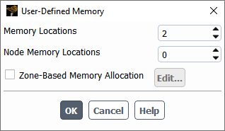
You must ensure that there are a sufficient number of UDMs for indexing. Otherwise, an error message is printed and the Python UDF will fail to load. For example, if a Python UDF accesses a UDM up to index 1, at least two UDMs should be defined in Fluent (see Figure 33.4: User-Defined Memory Dialog Box).
An example that uses UDMs is given below. It fills the 0th UDM using a function that evaluates spatially varying values, and the 1st UDM using a function that calculates velocity magnitude from the velocity components.
def udf_fill_udm0(c_centroid):
    x,y,z = c_centroid
    if y < 0.005:
        if x > 0.005:
            mag = 1.0
        else:
            mag = 2.0
    return Real(mag)

def udf_calc_vel_mag(c_u, c_v, c_w):
    # write velocity magnitude for postprocessing
    return math.sqrt(Real(c_u*c_u + c_v*c_v + c_w*c_w))

UDF.add_cell_zone_udm(udf_fill_udm0, 0)
UDF.add_cell_zone_udm(udf_calc_vel_mag, 1)
You can define a global reduction, as shown in the following example:
MAXT = UDF.reduce('max', c_t, [1])This defines a variable MAXT (a single floating-point value)
that can be used elsewhere by the Python code. Here, UDF.reduce
is a predefined function from the UDF module, and its arguments are:
'max'This is a string indicating the global reduction operation. The supported operations are
'min','max','avg', and'sum'.c_tThis is one of the predefined fields. For others, see Table 33.1: Supported Variables.
[1]This is a list of zone IDs to which the reduction applies.
After it is defined, this variable can be used in other UDF functions. Note that if a
function uses MAXT, that function must explicitly lists
MAXT as one of the function parameters; you cannot use
MAXT as a Python global variable.
Example
The following provides a detailed example that demonstrates the usage of global reduction. The case is a pseudo-2D channel with a square shaped obstacle in the middle. It has the following conditions:
The inlet (the left domain boundary, indicated using blue arrows, with a face zone ID equal to 6) has a cold fluid (T = 300K) that enters the domain at a uniform velocity profile of 0.5 m/s.
The cylinder (the hollow square in the domain with a face zone ID equal to 7) is heating up with time following a linear rule: T=300+100t [K].
An operation protocol is imposed, such that after the temperature in the fluid cell zone (with cell zone ID equal to 1) exceeds 305 K, the inlet velocity is doubled to 1.0 m/s.
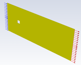
The three conditions are implemented in the Python UDF that follows. The code uses three zone IDs and imposes two transient boundary conditions, one of which involves global reduction, yet it has only 10 lines of code.
MAXT = UDF.reduce('max', c_t, [1])

def udf_cylinder_temperature(flow_time):
    return min(Real(310.0), Real(300.0 + 100.0 * flow_time))

def udf_velocity_profile(f_centroid, MAXT):
    if MAXT > Real(305.0):
        return (Real(1.0), Real(0), Real(0))
    else:
        return (Real(0.5), Real(0), Real(0))

UDF.add(udf_velocity_profile, 'boundary-condition', 'momentum', 'velocity', UDF.velocity_inlet_face_zones())
UDF.add(udf_cylinder_temperature, 'boundary-condition', 'energy', 'temperature', UDF.wall_face_zones())
Note that the cylinder temperature increases from T = 300 to 305 in 0.05 seconds. Because the thermal boundary layer takes some time to develop, the cell next to the hot cylinder reaches T = 305 after a short delay, then the inlet velocity increases from 0.5 m/s to 1.0 m/s. The time series of the maximum inlet velocity confirms this behavior (Figure 33.6: Time Series of the Maximum Inlet Velocity).
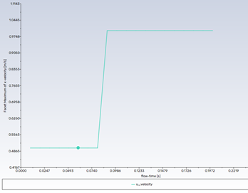
Notice that the maximum inlet velocity magnitude doubles after the maximum cell zone temperature exceeds a threshold specified in the Python UDF.
Due to the code transformation that takes place behind the scenes, it is not possible to interactively debug a Python UDF, in that you cannot open the Python UDF code in an integrated development environment (IDE) software, set a break point, and step through the code. You must instead run the case and check the results. The following tips are recommended for troubleshooting:
You should have a few small cases ready for testing the Python UDF. For example, you might want to specify the velocity profile at a pipe inlet: instead of using a case with millions of cells to write and test the Python UDF, it is much more efficient to use a small pipe case with only hundreds or thousands of cells.
You can insert the
printcommand in the Python UDF code, which prints data to the Fluent console. As an example, consider the implementation of a parabolic velocity profile for a pseudo-2D channel. You could use the code that follows:```python def udf_velocity_profile(f_centroid): y = f_centroid[1] u = (Real(1.0) - pow(y / Real(5), Real(2))) print(y, u) # the print statement return (u, Real(0), Real(0)) UDF.add(udf_velocity_profile, 'boundary-condition', 'momentum', 'velocity', [6]) ```The
printcommand is invoked at every face of the inlet zone (in this case, face zone6), and the result can be visualized using a program such as Matplotlib. Because the printing happens in a random order—a typical character of parallel execution—you can plot the data using a scatter plot instead of a line plot. You should use a case with a small number of faces to avoid printing excessive amount of messages in the console.
In this example, a Python UDF is applied at the inlet face zone (ID = 6). The u velocity component is calculated from the face centroid coordinate to impose a parabolic profile.
def udf_myconstant():
    return Real(0.5)

def udf_velocity_profile(f_centroid):
    return Real(0.5) + udf_myconstant() - pow(f_centroid[1]/Real(5), Real(2)), Real(0), Real(0)

# apply the velocity profile to zone 6
UDF.add_boundary_condition_velocity(udf_velocity_profile, [6])
This example also demonstrates the use of one UDF function within another UDF function.
Note: All function parameters (f_centroid, in this case) are read
only, and you should not modify their value in the function body. This restriction
applies to all other examples in the following sections and to Python UDFs in general.
To see an equivalent C UDF, see vprofile.c in Parabolic Velocity Inlet Profile in an Elbow Duct in the Fluent Customization Manual.
In this Python UDF example, the strain-rate magnitude is computed and used to determine the laminar viscosity.
def udf_visc(c_u_g, c_v_g, c_w_g):
dxx = c_u_g[0]
dyy = c_v_g[1]
dzz = c_w_g[2]
dxy = Real(0.5) * (c_u_g[1] + c_v_g[0])
dxz = Real(0.5) * (c_u_g[2] + c_w_g[0])
dyz = Real(0.5) * (c_v_g[2] + c_w_g[1])
strain_rate = math.sqrt(Real(2) * (dxx*dxx + dyy*dyy + dzz*dzz + Real(2)*(dxy*dxy + dxz*dxz + dyz*dyz)))
# Calculate viscosity
Eta0 = Real(0.1604)
Etainf = Real( 0.0674)
lam = Real(1.46e-3)
n0 = Real(0.5996)
one = Real(1)
two = Real(2)
return Etainf+(Eta0-Etainf) * pow(one + pow(lam*strain_rate, two), (n0-one)/two)
# add laminar viscosity UDF for all cell zones
UDF.add_laminar_viscosity(udf_visc, UDF.all_cell_zones())This Python UDF example calculates a transient energy source. The built-in variables
flow_time and c_centroid provide time
and cell-centroid coordinates, and Python's math module provides the mathematical function
(sin) and constant (pi).
def udf_heat_source(flow_time, c_centroid):
    x = c_centroid[0] + Real(0.02)
    y = c_centroid[1]
    radius = Real(0.003)
    mag = Real(0.0)
    omega = Real(2.0 * math.pi)

    if x*x + y*y < radius*radius:
        mag = Real(600.0) * math.sin(omega*flow_time)

    return mag

UDF.add_cell_zone_energy_source(udf_heat_source, [2])In this Python UDF example, the laminar viscosity is calculated as a piecewise-linear function of temperature.
def udf_visc(c_t):
    if c_t > Real(288.0):
        return Real(5.5e-3)
    elif c_t > Real(286.0):
        return Real(143.2135) - Real(0.49725)*c_t
    else:
        return Real(1.0)

UDF.add_laminar_viscosity(udf_visc, [1])
To see an equivalent C UDF, see Solidification via a Temperature-Dependent Viscosity in the Fluent Customization Manual.
The following Python UDF defines a time- and position-dependent inlet velocity boundary condition.
number_of_waves_per_yz = Real(3.0)

kx = Real(number_of_waves_per_yz*math.pi)
ky =-kx
kz = kx
ux = Real(2.0)/math.sqrt(Real(6.0))
uy = Real(0.5)*ux
uz = Real(0.5)*ux

Uin   = Real(30.0)
omega = kx * Uin

def udf_velocity_profile(flow_time, f_centroid):
    x, y, z = f_centroid[0], f_centroid[1], f_centroid[2]
    factor = math.cos(kx*x + ky*y + kz*z - omega*flow_time)
    u_prof = Uin + ux*factor
    v_prof =       uy*factor
    w_prof =       uz*factor
    return Real(u_prof), Real(v_prof), Real(w_prof)

UDF.add_boundary_condition_velocity(udf_velocity_profile, [5])The following Python UDF is for a pseudo-2D swirling flow created by a momentum source.
def udf_swirling_force(c_centroid):
x, y, z = c_centroid
radius = math.sqrt(x*x + y*y)
if radius < Real(0.001):
return Real(0.0), Real(0.0), Real(0.0)
return Real(-y/radius), Real(x/radius), Real(0.0)
UDF.add(udf_swirling_force, 'cell-zone-source', 'momentum', 'velocity', [2])Note that a momentum source term UDF is much simpler to implement in a Python UDF. For a UDF written in C, you have to implement the source term for each of the x, y, z components of the momentum equation, whereas in a Python UDF, you just need to implement a single UDF.
The recommended way to customize the Fluent GPU Solver is to use user-defined
functions (UDFs) written in Python, as described in Python User-Defined Functions (UDFs). If you must use UDFs written in C, you should note
that only the following DEFINE macros may potentially work with the
Fluent GPU Solver, and you must verify that they are performing as intended on an
individual basis.
Table 33.4: Potentially Supported DEFINE Macros for C UDFs
DEFINE Macros |
|---|
DEFINE_INIT |
DEFINE_EXECUTE_AFTER_CASE |
DEFINE_EXECUTE_AFTER_DATA |
DEFINE_EXECUTE_AT_EXIT |
DEFINE_EXECUTE_ON_LOADING |
DEFINE_ON_DEMAND |
DEFINE_PDF_TABLE |
DEFINE_PROFILE |
DEFINE_RW_FILE |
DEFINE_RW_HDF_FILE |
When loading a C UDF in the Fluent GPU Solver, Fluent checks the list of functions
in the UDF library and issues warnings in the console if DEFINE
macros are detected that are not in the previous list.