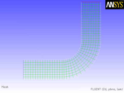
Consider the elbow duct illustrated in Figure 8.10: The Mesh for the Elbow Duct Example. The domain has a velocity inlet on the left side, and a pressure outlet at the top of the right side.

Figure 8.10: The Mesh for the Elbow Duct Example

A flow field in which a constant x velocity is applied at the inlet will be compared with one where a parabolic x velocity profile is applied. While the application of a profile using a piecewise-linear profile is available with the boundary profiles option, the specification of a polynomial can be accomplished only by a user-defined function.

The results of a constant velocity (of 0.1 m/sec) at the inlet are shown in Figure 8.11: Velocity Magnitude Contours for a Constant Inlet x Velocity and Figure 8.12: Velocity Vectors for a Constant Inlet x Velocity. The velocity profile is seen to develop as the flow passes through the duct.

Figure 8.11: Velocity Magnitude Contours for a Constant Inlet x Velocity

Figure 8.12: Velocity Vectors for a Constant Inlet x Velocity

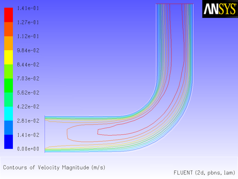
Now suppose that you want to impose a non-uniform x velocity to the duct inlet, which has a parabolic shape. The velocity is 0 m/s at the walls of the inlet and 0.1 m/s at the center.

A UDF is used to introduce this parabolic profile at the inlet. The C source code (vprofile.c) is shown below. The function makes use of Ansys Fluent-supplied solver functions that are described in Face Macros.

The UDF, named inlet_x_velocity, is defined using DEFINE_PROFILE and has two arguments: thread and position. Thread is a pointer to the face’s thread, and position is an integer that is a numerical label for the variable being set within each loop.

The function begins by declaring variable f as a face_t data type. A one-dimensional array x and variable y are declared as real data types. A looping macro is then used to loop over each face in the zone to create a profile, or an array of data. Within each loop, F_CENTROID outputs the value of the face centroid (array x) for the face with index f that is on the thread pointed to by thread. The y coordinate stored in x[1] is assigned to variable y, and is then used to calculate the x velocity. This value is then assigned to F_PROFILE, which uses the integer position (passed to it by the solver based on your selection of the UDF as the boundary condition for x velocity in the Velocity Inlet dialog box) to set the x velocity face value in memory.

/***********************************************************************
   vprofile.c 
  UDF for specifying steady-state velocity profile boundary condition
 ************************************************************************/
 
 #include "udf.h"
 
 DEFINE_PROFILE(inlet_x_velocity, thread, position)
 {
    real x[ND_ND]; /* this will hold the position vector */
    real y, h;
    face_t f;
    h = 0.016; /* inlet height in m */
    begin_f_loop(f,thread)
      {
        F_CENTROID(x, f, thread);
        y = 2.*(x[1]-0.5*h)/h; /* non-dimensional y coordinate */
        F_PROFILE(f, thread, position) = 0.1*(1.0-y*y);
      }
    end_f_loop(f, thread)
 } 

To make use of this UDF in Ansys Fluent, you will first need to interpret (or compile) the function, and then hook it to Ansys Fluent using the graphical user interface. Follow the procedure for interpreting source files using the Interpreted UDFs dialog box (Interpreting a UDF Source File Using the Interpreted UDFs Dialog Box), or compiling source files using the Compiled UDFs dialog box (Compiling a UDF Using the GUI).

To hook the UDF to Ansys Fluent as the velocity boundary condition for the zone of choice, open the Velocity Inlet dialog box and click the Momentum tab (Figure 8.13: The Velocity Inlet Dialog Box).

 Setup →   Boundary Conditions →   velocity-inlet → Edit...

Figure 8.13: The Velocity Inlet Dialog Box

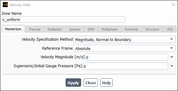
In the X-Velocity drop-down list, select udf inlet_x_velocity, the name that was given to the function above (with udf preceding it). Click OK to accept the new boundary condition and close the dialog box. Your user-defined profile will be used in the subsequent solution calculation.

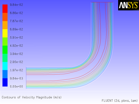
After the solution is initialized and run to convergence, a revised velocity field is obtained as shown in Figure 8.14: Velocity Magnitude Contours for a Parabolic Inlet x Velocity and Figure 8.15: Velocity Vectors for a Parabolic Inlet x Velocity. The velocity field shows a maximum at the center of the inlet, which drops to zero at the walls.

Figure 8.14: Velocity Magnitude Contours for a Parabolic Inlet x Velocity

Figure 8.15: Velocity Vectors for a Parabolic Inlet x Velocity

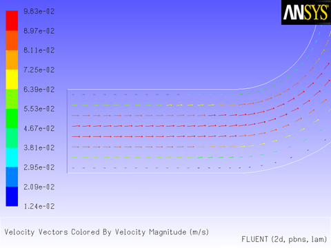
In this example, a temporally periodic pressure boundary condition will be applied to the outlet of a tube using a UDF. The pressure has the form

The tube is assumed to be filled with air, with a fixed total pressure at the inlet. The pressure of the air fluctuates at the outlet about an equilibrium value () of 101325 Pa, with an amplitude of 5 Pa and a frequency of 10 rad/s.

The source file listing for the UDF that describes the transient outlet profile is shown below. The function, named unsteady_pressure, is defined using the DEFINE_PROFILE macro. The utility CURRENT_TIME is used to look up the real flow time, which is assigned to the variable t. (See Time-Dependent Macros for details on CURRENT_TIME).

/**********************************************************************
   unsteady.c 
  UDF for specifying a transient pressure profile boundary condition
 ***********************************************************************/
 
 #include "udf.h"
 
 DEFINE_PROFILE(unsteady_pressure, thread, position)
 {
    face_t f;
    real t = CURRENT_TIME;
    begin_f_loop(f, thread)
      {
        F_PROFILE(f, thread, position) = 101325.0 + 5.0*sin(10.*t);
      }
    end_f_loop(f, thread)
   
 } 

Before you can interpret or compile the UDF, you must specify a transient flow calculation in the General task page. Then, follow the procedure for interpreting source files using the Interpreted UDFs dialog box (Interpreting a UDF Source File Using the Interpreted UDFs Dialog Box), or compiling source files using the Compiled UDFs dialog box (Compiling a UDF Using the GUI).

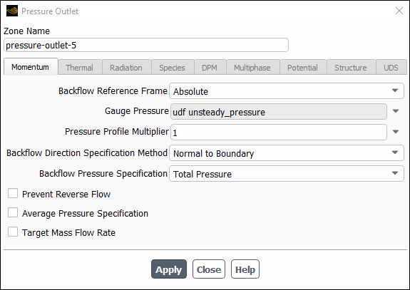
The sinusoidal pressure boundary condition defined by the UDF can now be hooked to the outlet zone. In the Pressure Outlet dialog box (Figure 8.16: The Pressure Outlet Dialog Box), simply select the name of the UDF given in this example with the word udf preceding it (udf unsteady_pressure) from the Gauge Pressure drop-down list. Click OK to accept the new boundary condition and close the dialog box. Your user-defined profile will be used in the subsequent solution calculation.

 Setup →   Boundary Conditions →   pressure-outlet-5 → Edit...

Figure 8.16: The Pressure Outlet Dialog Box

When a source term is being modeled with a UDF, it is important to understand the context in which the function is called. When you add a source term, Ansys Fluent will call your function as it performs a global loop on cells. Your function should compute the source term and return it to the solver.

In this example, a momentum source will be added to a 2D Cartesian duct flow. The duct is 4 m long and 2 m wide, and will be modeled using a symmetry boundary through the middle. Liquid metal (with properties listed in Table 8.1: Properties of the Liquid Metal) enters the duct at the left with a velocity of 1 mm/s at a temperature of 290 K. After the metal has traveled 0.5 m along the duct, it is exposed to a cooling wall, which is held at a constant temperature of 280 K. To simulate the freezing of the metal, a momentum source is applied to the metal as soon as its temperature falls below 288 K. The momentum source is proportional to the x component of the velocity, , and has the opposite sign:

(8–1)

where C is a constant. As the liquid cools, its motion will be reduced to zero, simulating the formation of the solid. (In this simple example, the energy equation will not be customized to account for the latent heat of freezing. The velocity field will be used only as an indicator of the solidification region.)

The solver linearizes source terms in order to enhance the stability and convergence of a solution. To allow the solver to do this, you need to specify the dependent relationship between the source and solution variables in your UDF, in the form of derivatives. The source term, , depends only on the solution variable, . Its derivative with respect to is

(8–2)

The following UDF specifies a source term and its derivative. The function, named cell_x_source, is defined on a cell using DEFINE_SOURCE. The constant C in Equation 8–1 is called CON in the function, and it is given a numerical value of 20 kg/-s, which will result in the desired units of N/ for the source. The temperature at the cell is returned by C_T(cell,thread). The function checks to see if the temperature is below (or equal to) 288 K. If it is, the source is computed according to Equation 8–1 (C_U returns the value of the x velocity of the cell). If it is not, the source is set to 0. At the end of the function, the appropriate value for the source is returned to the Ansys Fluent solver.

/******************************************************************
   UDF that adds momentum source term and derivative to duct flow
 *******************************************************************/
 
 #include "udf.h"
 
 #define CON 20.0
 
 DEFINE_SOURCE(cell_x_source, cell, thread, dS, eqn)
 {
    real source;
    if (C_T(cell,thread) <= 288.)
    {
      source = -CON*C_U(cell,thread);
      dS[eqn] = -CON;
    }
    else
    {
      source = dS[eqn] = 0.;
    }
    return source;
 } 

To make use of this UDF in Ansys Fluent, you will first need to interpret (or compile) the function, and then hook it to Ansys Fluent using the graphical user interface. Follow the procedure for interpreting source files using the Interpreted UDFs dialog box (Interpreting a UDF Source File Using the Interpreted UDFs Dialog Box), or compiling source files using the Compiled UDFs dialog box (Compiling a UDF Using the GUI).

To include source terms in the calculation, you will first need to open the Fluid dialog box (Figure 8.17: The Fluid Dialog Box) by selecting the fluid zone in the Cell Zone Conditions task page and clicking Edit....

 Setup →   Cell Zone Conditions →   fluid → Edit...

Figure 8.17: The Fluid Dialog Box

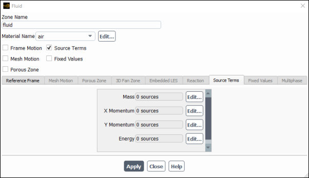
Enable the Source Terms option in the Fluid dialog box and click the Source Terms tab. This will display the momentum source term parameters in the scrollable window. Then, click the Edit... button next to the X Momentum source term to open the X Momentum sources dialog box (Figure 8.18: The X Momentum sources Dialog Box).

Figure 8.18: The X Momentum sources Dialog Box

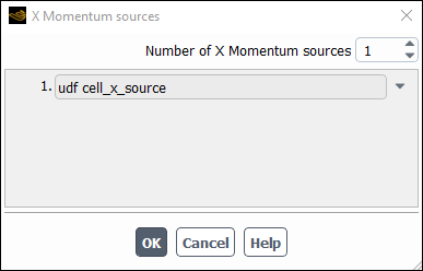
Enter 1 for the Number of Momentum sources in the X Momentum sources dialog box and then select the function name for the UDF (udf cell_x_source) in the drop-down list that appears. (Note that the name that is displayed in the drop-down lists is your UDF name preceded by the word udf.) Click OK to accept the new cell zone condition and close the dialog box. The X Momentum parameter in the Fluid dialog box will now display 1 source. Click OK to fix the new momentum source term for the solution calculation and close the Fluid dialog box.

After the solution has converged, you can view contours of static temperature to see the cooling effects of the wall on the liquid metal as it moves through the duct (Figure 8.19: Temperature Contours Illustrating Liquid Metal Cooling).

Figure 8.19: Temperature Contours Illustrating Liquid Metal Cooling

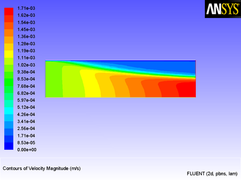
Contours of velocity magnitude (Figure 8.20: Velocity Magnitude Contours Suggesting Solidification) show that the liquid in the cool region near the wall has indeed come to rest to simulate solidification taking place.

Figure 8.20: Velocity Magnitude Contours Suggesting Solidification

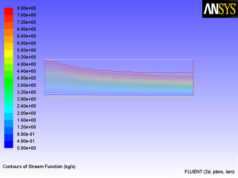
The solidification is further illustrated by line contours of stream function (Figure 8.21: Stream Function Contours Suggesting Solidification).

Figure 8.21: Stream Function Contours Suggesting Solidification

To more accurately predict the freezing of a liquid in this manner, an energy source term would be needed, as would a more accurate value for the constant appearing in Equation 8–1.

UDFs for properties (as well as sources) are called from within a loop on cells. For this reason, functions that specify properties are required to compute the property for only a single cell, and return the value to the Ansys Fluent solver.

The UDF in this example generates a variable viscosity profile to simulate solidification, and is applied to the same problem that was presented in Adding a Momentum Source to a Duct Flow. The viscosity in the warm ( K) fluid has a molecular value for the liquid (5.5 kg/m-s), while the viscosity for the cooler region ( 286 K) has a much larger value (1.0 kg/m-s). In the intermediate temperature range (286 K 288 K), the viscosity follows a linear profile (Equation 8–3) that extends between the two values given above:

(8–3)

This model is based on the assumption that as the liquid cools and rapidly becomes more viscous, its velocity will decrease, thereby simulating solidification. Here, no correction is made for the energy field to include the latent heat of freezing. The C source code for the UDF is shown below.

The function, named cell_viscosity, is defined on a cell using DEFINE_PROPERTY. Two real variables are introduced: temp, the value of C_T(cell,thread) , and mu_lam, the laminar viscosity computed by the function. The value of the temperature is checked, and based upon the range into which it falls, the appropriate value of mu_lam is computed. At the end of the function, the computed value for mu_lam is returned to the solver.

/*********************************************************************
   UDF for specifying a temperature-dependent viscosity property
 **********************************************************************/
 
 #include "udf.h"
 
 DEFINE_PROPERTY(cell_viscosity, cell, thread)
 {
    real mu_lam;
    real temp = C_T(cell, thread);
    if (temp > 288.)
     mu_lam = 5.5e-3;
    else if (temp > 286.)
     mu_lam = 143.2135 - 0.49725 * temp;
    else
     mu_lam = 1.;
    return mu_lam;
 } 

This function can be executed as an interpreted or compiled UDF in Ansys Fluent. Follow the procedure for interpreting source files using the Interpreted UDFs dialog box (Interpreting a UDF Source File Using the Interpreted UDFs Dialog Box), or compiling source files using the Compiled UDFs dialog box (Compiling a UDF Using the GUI).

To make use of the user-defined property in Ansys Fluent, you will need to open the Create/Edit Materials dialog box (Figure 8.22: The Create/Edit Materials Dialog Box) by selecting the liquid metal material in the Materials task page and clicking the Create/Edit... button.

 Setup →   Materials →   liquid_metal → Create/Edit...

Figure 8.22: The Create/Edit Materials Dialog Box

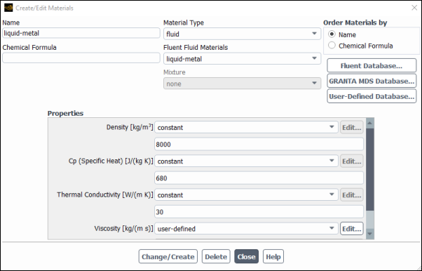
In the Create/Edit Materials dialog box, select user-defined in the drop-down list for Viscosity. This will open the User-Defined Functions dialog box (Figure 8.23: The User-Defined Functions Dialog Box), from which you can select the appropriate function name. In this example, only one option is available, but in other examples, you may have several functions from which to choose. (Recall that if you need to compile more than one interpreted UDF, the functions can be concatenated in a single source file prior to compiling.)

Figure 8.23: The User-Defined Functions Dialog Box

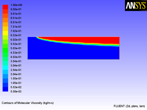
The results of this model are similar to those obtained in Adding a Momentum Source to a Duct Flow. Figure 8.24: Laminar Viscosity Generated by a User-Defined Function shows the viscosity field resulting from the application of the user-defined function. The viscosity varies rapidly over a narrow spatial band from a constant value of 0.0055 to 1.0 kg/m-s.

The velocity field (Figure 8.25: Contours of Velocity Magnitude Resulting from a User-Defined Viscosity) demonstrates that the liquid slows down in response to the increased viscosity, as expected. In this model, there is a large "mushy" region, in which the motion of the fluid gradually decreases. This is in contrast to the first model, in which a momentum source was applied and a more abrupt change in the fluid motion was observed.

Figure 8.24: Laminar Viscosity Generated by a User-Defined Function

Figure 8.25: Contours of Velocity Magnitude Resulting from a User-Defined Viscosity

Figure 8.26: Stream Function Contours Suggesting Solidification

A custom volume reaction rate for a simple system of two gaseous species is considered. The species are named species-a and species-b. The reaction rate is one that converts species-a into species-b at a rate given by the following expression:

(8–4)

where is the mass fraction of species-a, and and are constants.

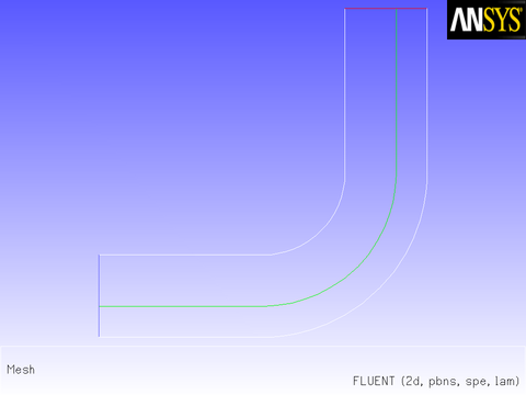
The 2D (planar) domain consists of a 90° bend. The duct has a porous region covering the bottom and right-hand wall, and the reaction takes place in the porous region only. The species in the duct have identical properties. The density is 1.0 kg/, and the viscosity is 1.7894 kg/m-s.

The outline of the domain is shown in Figure 8.27: The Outline of the 2D Duct. The porous medium is the region below and to the right of the line that extends from the inlet on the left to the pressure outlet at the top of the domain.

Figure 8.27: The Outline of the 2D Duct

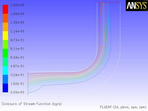
Through the inlet on the left, gas that is purely species-a enters with an x velocity of 0.1 m/s. The gas enters both the open region on the top of the porous medium and the porous medium itself, where there is an inertial resistance of 5 m^-1 in each of the two coordinate directions. The laminar flow field (Figure 8.28: Streamlines for the 2D Duct with a Porous Region) shows that most of the gas is diverted from the porous region into the open region.

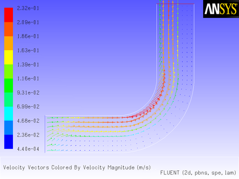
The flow pattern is further substantiated by the vector plot shown in Figure 8.29: Velocity Vectors for the 2D Duct with a Porous Region. The flow in the porous region is considerably slower than that in the open region.

Figure 8.28: Streamlines for the 2D Duct with a Porous Region

Figure 8.29: Velocity Vectors for the 2D Duct with a Porous Region

The source code (rate.c) that contains the UDF used to model the reaction taking place in the porous region is shown below. The function, named vol_reac_rate, is defined on a cell for a given species mass fraction using DEFINE_VR_RATE. The UDF performs a test to check if a zone is porous, so that the reaction rate is only calculated for the porous zone. This is done to save calculation time. Note that, in calculating the reaction source terms, Fluent will always use the actual fluid volume for a reacting zone, so there is no need to multiply the volumetric rate by porosity. This will be done by Fluent internally. The macro FLUID_THREAD_P(t) is used to determine if a cell thread is a fluid (rather than a solid) thread. The variable THREAD_VAR(t).fluid.porous is used to check if a fluid cell thread is a porous region.

/******************************************************************
   rate.c 
  Compiled UDF for specifying a reaction rate in a porous medium
 *******************************************************************/
 
 #include "udf.h"
 
 #define K1 2.0e-2
 #define K2 5.
 
 DEFINE_VR_RATE(vol_reac_rate,c,t,r,mole_weight,species_mf,rate,rr_t)
 {
    real s1 = species_mf[0];
    real mw1 = mole_weight[0];
    if (FLUID_THREAD_P(t) && THREAD_VAR(t).fluid.porous)
      *rate = K1*s1/pow((1.+K2*s1),2.0)/mw1;
    else
      *rate = 0.;
    *rr_t = *rate;
 } 

This UDF is executed as a compiled UDF in Ansys Fluent. Follow the procedure for compiling source files using the Compiled UDFs dialog box that is described in Compiling a UDF Using the GUI.

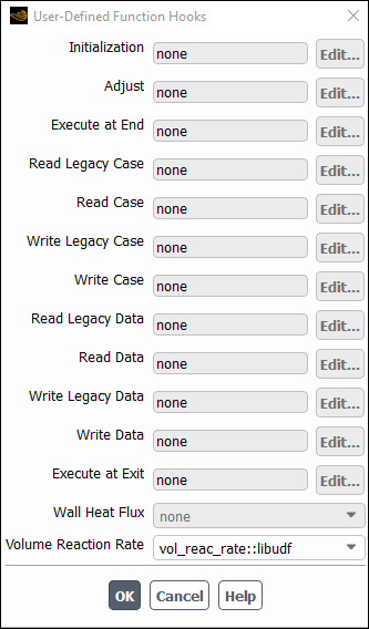
After the function vol_reac_rate is compiled and loaded, you can hook the reaction rate UDF to Ansys Fluent by selecting the function’s name in the Volume Reaction Rate Function drop-down list in the User-Defined Function Hooks dialog box (Figure 6.75: The User-Defined Function Hooks Dialog Box).

 Parameters & Customization → User Defined Functions  Function Hooks...

Figure 8.30: The User-Defined Functions Hooks Dialog Box

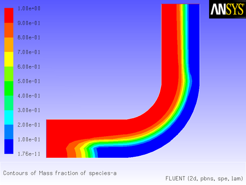
Initialize and run the calculation. The converged solution for the mass fraction of species-a is shown in Figure 8.31: Mass Fraction for species-a Governed by a Reaction in a Porous Region. The gas that moves through the porous region is gradually converted to species-b in the horizontal section of the duct. No reaction takes place in the fluid region, although some diffusion of species-b out of the porous region is suggested by the wide transition layer between the regions of 100% and 0% species-a.

Figure 8.31: Mass Fraction for species-a Governed by a Reaction in a Porous Region

Below is an example of a compiled UDF that computes the gradient of temperature to the fourth power, and stores its magnitude in a user-defined scalar. The computed temperature gradient can, for example, be subsequently used to plot contours. Although the practical application of this UDF is questionable, its purpose here is to show the methodology of computing gradients of arbitrary quantities that can be used for postprocessing.

/***********************************************************************/
/* UDF for computing the magnitude of the gradient of T^4                    */
/***********************************************************************/
 
 #include "udf.h"
 
 /* Define which user-defined scalars to use. */
 enum
 {
    T4,
    MAG_GRAD_T4,
    N_REQUIRED_UDS
 };
 
 DEFINE_ADJUST(adjust_fcn, domain)
 {
    Thread *t;
    cell_t c;
    face_t f;
 
    /* Make sure there are enough user-defined scalars. */
    if (n_uds < N_REQUIRED_UDS)
      Internal_Error("not enough user-defined scalars allocated");
      /* Fill first UDS with temperature raised to fourth power. */
      thread_loop_c (t,domain)
        {
           if (NULL != THREAD_STORAGE(t,SV_UDS_I(T4)))
           {
            begin_c_loop (c,t)
            {
             real T = C_T(c,t);
             C_UDSI(c,t,T4) = pow(T,4.);
            }
            end_c_loop (c,t)
           }
        }
 
      thread_loop_f (t,domain)
        {
         if (NULL != THREAD_STORAGE(t,SV_UDS_I(T4)))
           {
            begin_f_loop (f,t)
              {
               real T = 0.;
               if (NULL != THREAD_STORAGE(t,SV_T))
                 T = F_T(f,t);
               else if (NULL != THREAD_STORAGE(t->t0,SV_T))
                 T = C_T(F_C0(f,t),t->t0);
                 F_UDSI(f,t,T4) = pow(T,4.);
                }
            end_f_loop (f,t)
           }
          }
      /* Fill second UDS with magnitude of gradient. */
      thread_loop_c (t,domain)
        {
         if (NULL != THREAD_STORAGE(t,SV_UDS_I(T4)) &&
            NULL != T_STORAGE_R_NV(t,SV_UDSI_G(T4)))
          {
            begin_c_loop (c,t)
            {
             C_UDSI(c,t,MAG_GRAD_T4) = NV_MAG(C_UDSI_G(c,t,T4));
            }
            end_c_loop (c,t)
         }
        }
      thread_loop_f (t,domain)
      {
       if (NULL != THREAD_STORAGE(t,SV_UDS_I(T4)) &&
          NULL != T_STORAGE_R_NV(t->t0,SV_UDSI_G(T4)))
        {
          begin_f_loop (f,t)
           {
              F_UDSI(f,t,MAG_GRAD_T4)=C_UDSI(F_C0(f,t),t->t0,MAG_GRAD_T4);
           }
          end_f_loop (f,t)
       }
    }
 } 

The conditional statement if (NULL != THREAD_STORAGE(t,SV_UDS_I(T4))) is used to check if the storage for the user-defined scalar with index T4 has been allocated, while NULL != T_STORAGE_R_NV(t,SV_UDSI_G(T4)) checks whether the storage of the gradient of the user-defined scalar with index T4 has been allocated.

In addition to compiling this UDF, as described in Compiling UDFs, you will need to enable the solution of a user-defined scalar transport equation in Ansys Fluent.

 Parameters & Customization → User Defined Scalars  New...

See User-Defined Scalar (UDS) Transport Equations in the Fluent Theory Guide for UDS equation theory and details on how to set up scalar equations.

This section provides an example that demonstrates how the P1 radiation model can be implemented as a UDF, utilizing a user-defined scalar transport equation. In the P1 model, the variation of the incident radiation, G, in the domain can be described by an equation that consists of a diffusion and source term.

The transport equation for incident radiation, G, is given by Equation 8–5. The diffusion coefficient, Γ, is given by Equation 8–6 and the source term is given by Equation 8–7. See P-1 Radiation Model Theory in the Fluent Theory Guide for more details.

(8–5)

(8–6)

(8–7)

The boundary condition for G at the walls is equal to the negative of the radiative wall heat flux, (Equation 8–8), where is the outward normal vector (see P-1 Radiation Model Theory in the Fluent Theory Guide for more details). The radiative wall heat flux can be given by Equation 8–9.

(8–8)

(8–9)

This form of the boundary condition is unfortunately specified in terms of the incident radiation at the wall, . This mixed boundary condition can be avoided by solving first for using Equation 8–8 and Equation 8–9, resulting in Equation 8–10. Then, this expression for is substituted back into Equation 8–9 to give the radiative wall heat flux as Equation 8–11.

(8–10)

(8–11)

The additional and terms that appear in Equation 8–10 and Equation 8–11 are a result of the evaluation of the gradient of incident radiation in Equation 8–8.

In Ansys Fluent, the component of a gradient of a scalar directed normal to a cell boundary (face), n, is estimated as the sum of primary and secondary components. The primary component represents the gradient in the direction defined by the cell centroids, and the secondary component is in the direction along the face separating the two cells. From this information, the face normal component can be determined. The secondary component of the gradient can be found using the Ansys Fluent macro BOUNDARY_SECONDARY_GRADIENT_SOURCE (which is described in Boundary Secondary Gradient Source (BOUNDARY_SECONDARY_GRADIENT_SOURCE)). The use of this macro first requires that cell geometry information be defined, which can be readily obtained by the use of a second macro, BOUNDARY_FACE_GEOMETRY (see Boundary Face Geometry (BOUNDARY_FACE_GEOMETRY)). You will see these macros called in the UDF that defines the wall boundary condition for G.

To complete the implementation of the P1 model, the radiation energy equation must be coupled with the thermal energy equation. This is accomplished by modifying the source term and wall boundary condition of the energy equation. Consider first how the energy equation source term must be modified. The gradient of the incident radiation is proportional to the radiative heat flux. A local increase (or decrease) in the radiative heat flux is attributable to a local decrease (or increase) in thermal energy via the absorption and emission mechanisms. The gradient of the radiative heat flux is therefore a (negative) source of thermal energy. The source term for the incident radiation Equation 8–7 is equal to the gradient of the radiative heat flux and hence its negative specifies the source term needed to modify the energy equation (see P-1 Radiation Model Theory in the Fluent Theory Guide for more details).

Now consider how the energy boundary condition at the wall must be modified. Locally, the only mode of energy transfer from the wall to the fluid that is accounted for by default is conduction. With the inclusion of radiation effects, radiative heat transfer to and from the wall must also be accounted for. (This is done automatically if you use Ansys Fluent’s built-in P1 model.) The DEFINE_HEAT_FLUX macro allows the wall boundary condition to be modified to accommodate this second mode of heat transfer by specifying the coefficients of the equation discussed in DEFINE_HEAT_FLUX . The net radiative heat flux to the wall has already been given as Equation 8–9. Comparing this equation with that for in DEFINE_HEAT_FLUX will result in the proper coefficients for .

In this example, the implementation of the P1 model can be accomplished through six separate UDFs. They are all included in a single source file, which can be executed as a compiled UDF. The single user-defined scalar transport equation for incident radiation, G, uses a DEFINE_DIFFUSIVITY UDF to define Γ of Equation 8–6, and a UDF to define the source term of Equation 8–7. The boundary condition for at the walls is handled by assigning, in DEFINE_PROFILE, the negative of Equation 8–11 as the specified flux. A DEFINE_ADJUST UDF is used to instruct Ansys Fluent to check that the proper number of user-defined scalars has been defined (in the solver). Lastly, the energy equation must be assigned a source term equal to the negative of that used in the incident radiation equation and the DEFINE_HEAT_FLUX UDF is used to alter the boundary conditions at the walls for the energy equation.

In the solver, at least one user-defined scalar (UDS) equation must be enabled. The scalar diffusivity is assigned in the Create/Edit Materials dialog box for the scalar equation. The scalar source and energy source terms are assigned in the boundary condition dialog box for the fluid zones. The boundary condition for the scalar equation at the walls is assigned in the boundary condition dialog box for the wall zones. The DEFINE_ADJUST and DEFINE_HEAT_FLUX functions are assigned in the User-Defined Function Hooks dialog box.

Note that the residual monitor for the UDS equation should be reduced from to before running the solution. If the solution diverges, then it may be due to the large source terms. In this case, the under-relaxation factor should be reduced to and the solution re-run.

 /**************************************************************/
 /* Implementation of the P1 model using user-defined scalars  */
 /**************************************************************/
 
 #include "udf.h"
 #include "sg.h"
 
 /* Define which user-defined scalars to use. */
 enum
 {
    P1,
    N_REQUIRED_UDS
 };
 
 
 static real abs_coeff = 0.2; /* absorption coefficient */
 static real scat_coeff = 0.0;  /* scattering coefficient */
 static real las_coeff = 0.0; /* linear-anisotropic  */
               /* scattering coefficient */
 static real epsilon_w = 1.0; /* wall emissivity */
 
 
 DEFINE_ADJUST(p1_adjust, domain)
 {
    /* Make sure there are enough user defined-scalars. */
    if (n_uds < N_REQUIRED_UDS)
      Internal_Error("not enough user-defined scalars allocated");
 }
 
 
 DEFINE_SOURCE(energy_source, c, t, dS, eqn)
 {
    dS[eqn] = -16.*abs_coeff*SIGMA_SBC*pow(C_T(c,t),3.);
    return -abs_coeff*(4.*SIGMA_SBC*pow(C_T(c,t),4.) - C_UDSI(c,t,P1)); }
 
 
DEFINE_SOURCE(p1_source, c, t, dS, eqn)
{
   dS[eqn] = -abs_coeff;
   return abs_coeff*(4.*SIGMA_SBC*pow(C_T(c,t),4.) - C_UDSI(c,t,P1));
}
 
 
 DEFINE_DIFFUSIVITY(p1_diffusivity, c, t, i)
 {
    return 1./(3.*abs_coeff + (3. - las_coeff)*scat_coeff);
 }
 
 
 DEFINE_PROFILE(p1_bc, thread, position)
 
 {
    face_t f;
    real A[ND_ND],At;
    real dG[ND_ND],dr0[ND_ND],es[ND_ND],ds,A_by_es;
    real aterm,alpha0,beta0,gamma0,Gsource,Ibw;
    real Ew = epsilon_w/(2.*(2. - epsilon_w));
    Thread *t0=thread->t0;
    /* Do nothing if areas are not computed yet or not next to fluid. */
    if (!Data_Valid_P() || !FLUID_THREAD_P(t0)) return;
      begin_f_loop (f,thread)
      {
         cell_t c0 = F_C0(f,thread);
         BOUNDARY_FACE_GEOMETRY(f,thread,A,ds,es,A_by_es,dr0);
         At = NV_MAG(A);
         if (NULLP(T_STORAGE_R_NV(t0,SV_UDSI_G(P1))))
           Gsource = 0.;  /* if gradient not stored yet */
         else
           BOUNDARY_SECONDARY_GRADIENT_SOURCE(Gsource,SV_UDSI_G(P1),
                   dG,es,A_by_es,1.);
         gamma0 = C_UDSI_DIFF(c0,t0,P1);
         alpha0 = A_by_es/ds;
         beta0 = Gsource/alpha0;
         aterm = alpha0*gamma0/At;
         Ibw = SIGMA_SBC*pow(WALL_TEMP_OUTER(f,thread),4.)/M_PI;
         /* Specify the radiative heat flux. */
         F_PROFILE(f,thread,position) =
             aterm*Ew/(Ew + aterm)*(4.*M_PI*Ibw - C_UDSI(c0,t0,P1) + beta0);
      }
    end_f_loop (f,thread)
 }
 
 
 DEFINE_HEAT_FLUX(heat_flux, f, t, c0, t0, cid, cir)
 {
    real Ew = epsilon_w/(2.*(2. - epsilon_w));
    cir[0] = Ew * F_UDSI(f,t,P1);
  cir[3] = 4.0 * Ew * SIGMA_SBC;
 
 } 

This section describes another example of a user-defined real gas model. You can use this example as the basis for your own UDRGM code. In this example, the Redlich-Kwong equation of state is used in the UDRGM.

This section summarizes the equations used in developing the UDRGM for the Redlich-Kwong equation of state. The model is based on a modified form of the Redlich-Kwong equation of state described in [1]. The equations used in this UDRGM will be listed in the sections below.

The following nomenclature applies to this section:

The superscript 0 designates a reference state, and the subscript designates a critical point property.

The Redlich-Kwong equation of state can be written in the following form:

(8–12)

where

(8–13)

Since the real gas model in Ansys Fluent requires a function for density as a function of pressure and temperature, Equation 8–12 must be solved for the specific volume (from which the density can be easily obtained). For convenience, Equation 8–12 can be written as a cubic equation for specific volume as follows:

(8–14)

where

(8–15)

Equation 8–14 is solved using a standard algorithm for cubic equations (see [11] for details). In the UDRGM code, the cubic solution is coded to minimize the number of floating point operations. This is critical for optimal performance, since this function gets called numerous times during an iteration cycle.

It should be noted that the value of the exponent, , in the function will depend on the substance. A table of values can be found in [1] for some common substances. Alternatively, [1] states that values of are well correlated by the empirical equation

(8–16)

where is the acentric factor, defined as

(8–17)

In the above equation, is the saturated vapor pressure evaluated at temperature .

The derivatives of specific volume with respect to temperature and pressure can be easily determined from Equation 8–12 using implicit differentiation. The results are presented below:

(8–18)

(8–19)

where

(8–20)

The derivatives of density can be obtained from the above using the relations

(8–21)

(8–22)

Following [1], enthalpy for a real gas can be written

(8–23)

where is the enthalpy function for a thermally perfect gas (that is, enthalpy is a function of temperature alone). In the present case, a fourth-order polynomial for the specific heat for a thermally perfect gas [8] is employed:

(8–24)

and obtain the enthalpy from the basic relation

(8–25)

The result is

(8–26)

Note that is the enthalpy at a reference state , which can be chosen arbitrarily.

The specific heat for the real gas can be obtained by differentiating Equation 8–23 with respect to temperature (at constant pressure): becomes

(8–27)

The result is

(8–28)

Finally, the derivative of enthalpy with respect to pressure (at constant temperature) can be obtained using the following thermodynamic relation [8]:

(8–29)

Following [1], the entropy can be expressed in the form

(8–30)

where the superscript again refers to a reference state where the ideal gas law is applicable. For an ideal gas at a fixed reference pressure, , the entropy is given by

(8–31)

Note that the pressure term is zero since the entropy is evaluated at the reference pressure. Using the polynomial expression for specific heat, Equation 8–24, Equation 8–31 becomes

(8–32)

where is a constant, which can be absorbed into the reference entropy .

The speed of sound for a real gas can be determined from the thermodynamic relation

(8–33)

Noting that,

(8–34)

we can write the speed of sound as

(8–35)

The dynamic viscosity of a gas or vapor can be estimated using the following formula from [2]:

(8–36)

Here, is the reduced temperature

(8–37)

and is the molecular weight of the gas. This formula neglects the effect of pressure on viscosity, which usually becomes significant only at very high pressures.

Knowing the viscosity, the thermal conductivity can be estimated using the Eucken formula [4]:

(8–38)

It should be noted that both Equation 8–36 and Equation 8–38 are simple relations, and therefore may not provide satisfactory values of viscosity and thermal conductivity for certain applications. You are encouraged to modify these functions in the UDRGM source code if alternate formulae are available for a given gas.

Using the Redlich-Kwong Real Gas UDRGM simply requires the modification of the top block of #define macros to provide the appropriate parameters for a given substance. An example listing for is given below. The parameters required are:

The coefficients for the ideal gas specific heat polynomial were obtained from [8] (coefficients for other substances are also provided in [8]). After the source listing is modified, the UDRGM C code can be recompiled and loaded into Ansys Fluent in the manner described earlier.

/* The variables below need to be set for a particular gas */
 
 /* CO2 */
 
 /* REAL GAS EQUATION OF STATE MODEL - BASIC VARIABLES */
 /* ALL VARIABLES ARE IN SI UNITS! */
 
 #define RGASU UNIVERSAL_GAS_CONSTANT
 #define PI 3.141592654
 
 #define MWT 44.01
 #define PCRIT 7.3834e6
 #define TCRIT 304.21
 #define ZCRIT 0.2769
 #define VCRIT 2.15517e-3
 #define NRK 0.77
 
 /* IDEAL GAS SPECIFIC HEAT CURVE FIT */
 
 #define CC1 453.577
 #define CC2 1.65014
 #define CC3 -1.24814e-3
 #define CC4 3.78201e-7
 #define CC5 0.00
 
 /* REFERENCE STATE */
 
 #define P_REF 101325
 #define T_REF 288.15 

/**************************************************************/
/*                                                            */
/* User-Defined Function: Redlich-Kwong Equation of State     */
/*            for Real Gas Modeling                           */
/*                                                            */
/* Author: Frank Kelecy                                       */
/*  Date: May 2003                                            */
/* Version: 1.02                                              */
/*                                                            */
/* This implementation is completely general.                 */
/* Parameters set for CO2.                                    */
/*                                                            */
/**************************************************************/

#include "udf.h"
#include "stdio.h"
#include "ctype.h"
#include "stdarg.h"

/* The variables below need to be set for a particular gas */

/* CO2 */

/* REAL GAS EQUATION OF STATE MODEL - BASIC VARIABLES */
/* ALL VARIABLES ARE IN SI UNITS! */

#define RGASU UNIVERSAL_GAS_CONSTANT
#define PI  3.141592654

#define MWT 44.01
#define PCRIT 7.3834e6
#define TCRIT 304.21
#define ZCRIT 0.2769
#define VCRIT 2.15517e-3
#define NRK 0.77

/* IDEAL GAS SPECIFIC HEAT CURVE FIT */

#define CC1 453.577
#define CC2 1.65014
#define CC3 -1.24814e-3
#define CC4 3.78201e-7
#define CC5 0.00

/* REFERENCE STATE */

#define P_REF 101325
#define T_REF 288.15

/* OPTIONAL REFERENCE (OFFSET) VALUES FOR ENTHALPY AND ENTROPY */

#define H_REF 0.0
#define S_REF 0.0

static int (*usersMessage)(const char *,...);
static void (*usersError)(const char *,...);

/* Static variables associated with Redlich-Kwong Model */

static double rgas, a0, b0, c0, bb, cp_int_ref;


DEFINE_ON_DEMAND(I_do_nothing)
{
   /* this is a dummy function to allow us */
   /* to use the compiled UDFs utility   */
}

/*------------------------------------------------------------*/
/* FUNCTION: RKEOS_Setup                                      */
/*------------------------------------------------------------*/

void RKEOS_Setup(Domain *domain, cxboolean vapor_phase, char *species_list,
                 int(*messagefunc)(const char *format,...),
                 void (*errorfunc)(const char *format,...))
{

  rgas = RGASU/MWT;
  a0 = 0.42747*rgas*rgas*TCRIT*TCRIT/PCRIT;
  b0 = 0.08664*rgas*TCRIT/PCRIT;
  c0 = rgas*TCRIT/(PCRIT+a0/(VCRIT*(VCRIT+b0)))+b0-VCRIT;
  bb = b0-c0;
  cp_int_ref = CC1*log(T_REF)+T_REF*(CC2+
             T_REF*(0.5*CC3+T_REF*(0.333333*CC4+0.25*CC5*T_REF)));

  usersMessage = messagefunc;
  usersError = errorfunc;
  usersMessage("\nLoading Redlich-Kwong Library: %s\n", species_list);
}

/*------------------------------------------------------------*/
/* FUNCTION: RKEOS_pressure                                   */
/*      Returns pressure given T and density                  */
/*------------------------------------------------------------*/

double RKEOS_pressure(double temp, double density)
{
    double v = 1./density;
    double afun = a0*pow(TCRIT/temp,NRK);
    return rgas*temp/(v-bb)-afun/(v*(v+b0));
}

/*------------------------------------------------------------*/
/* FUNCTION: RKEOS_spvol                                      */
/*      Returns specific volume given T and P                 */
/*------------------------------------------------------------*/

double RKEOS_spvol(double temp, double press)
{
    double a1,a2,a3;
    double vv,vv1,vv2,vv3;
    double qq,qq3,sqq,rr,tt,dd;
    double afun = a0*pow(TCRIT/temp,NRK);

    a1 = c0-rgas*temp/press;
    a2 = -(bb*b0+rgas*temp*b0/press-afun/press);
    a3 = -afun*bb/press;

    /* Solve cubic equation for specific volume */

    qq = (a1*a1-3.*a2)/9.;
    rr = (2*a1*a1*a1-9.*a1*a2+27.*a3)/54.;
    qq3 = qq*qq*qq;
    dd = qq3-rr*rr;

  /* If dd < 0, then we have one real root */
  /* If dd >= 0, then we have three roots -> choose largest root */

  if (dd < 0.) {
     tt = pow(sqrt(-dd)+fabs(rr),0.333333);
     vv = (tt+qq/tt)-a1/3.;
  } else {
     tt = acos(rr/sqrt(qq3));
     sqq = sqrt(qq);
     vv1 = -2.*sqq*cos(tt/3.)-a1/3.;
     vv2 = -2.*sqq*cos((tt+2.*PI)/3.)-a1/3.;
     vv3 = -2.*sqq*cos((tt+4.*PI)/3.)-a1/3.;
     vv = (vv1 > vv2) ? vv1 : vv2;
     vv = (vv > vv3) ? vv : vv3;
  }

  return vv;
}

/*------------------------------------------------------------*/
/* FUNCTION: RKEOS_density                                    */
/*      Returns density given T and P                         */
/*------------------------------------------------------------*/

double RKEOS_density(cell_t cell, Thread *thread, cxboolean vapor_phase, double temp, double press, double yi[])
{
    return 1./RKEOS_spvol(temp, press); /* (Kg/m3) */
}

/*------------------------------------------------------------*/
/* FUNCTION: RKEOS_dvdp                                       */
/*      Returns dv/dp given T and rho                         */
/*------------------------------------------------------------*/

double RKEOS_dvdp(double temp, double density)
{
    double a1,a2,a1p,a2p,a3p,v,press;
    double afun = a0*pow(TCRIT/temp,NRK);

    press = RKEOS_pressure(temp, density);
    v = 1./density;

    a1 = c0-rgas*temp/press;
    a2 = -(bb*b0+rgas*temp*b0/press-afun/press);
    a1p = rgas*temp/(press*press);
    a2p = a1p*b0-afun/(press*press);
    a3p = afun*bb/(press*press);

    return -(a3p+v*(a2p+v*a1p))/(a2+v*(2.*a1+3.*v));
}

/*------------------------------------------------------------*/
/* FUNCTION: RKEOS_dvdt                                       */
/*      Returns dv/dT given T and rho                         */
/*------------------------------------------------------------*/

double RKEOS_dvdt(double temp, double density)
{
    double a1,a2,dadt,a1t,a2t,a3t,v,press;
    double afun = a0*pow(TCRIT/temp,NRK);

    press = RKEOS_pressure(temp, density);
    v = 1./density;

    dadt = -NRK*afun/temp;
    a1 = c0-rgas*temp/press;
    a2 = -(bb*b0+rgas*temp*b0/press-afun/press);
    a1t = -rgas/press;
    a2t = a1t*b0+dadt/press;
    a3t = -dadt*bb/press;

    return -(a3t+v*(a2t+v*a1t))/(a2+v*(2.*a1+3.*v));
}

/*------------------------------------------------------------*/
/* FUNCTION: RKEOS_Cp_ideal_gas                               */
/*      Returns ideal gas specific heat given T               */
/*------------------------------------------------------------*/

double RKEOS_Cp_ideal_gas(double temp)
{
    return (CC1+temp*(CC2+temp*(CC3+temp*(CC4+temp*CC5))));
}

/*------------------------------------------------------------*/
/* FUNCTION: RKEOS_H_ideal_gas                                */
/*      Returns ideal gas specific enthalpy given T           */
/*------------------------------------------------------------*/

double RKEOS_H_ideal_gas(double temp)
{
    return temp*(CC1+temp*(0.5*CC2+temp*(0.333333*CC3+
              temp*(0.25*CC4+temp*0.2*CC5))));
}

/*------------------------------------------------------------*/
/* FUNCTION: RKEOS_specific_heat                              */
/*      Returns specific heat given T and rho                 */
/*------------------------------------------------------------*/

double RKEOS_specific_heat(cell_t cell, Thread *thread, double temp, double density, double P, double yi[])
{
    double delta_Cp,press,v,dvdt,dadt;
    double afun = a0*pow(TCRIT/temp,NRK);

    press = RKEOS_pressure(temp, density);
    v = 1./density;
    dvdt = RKEOS_dvdt(temp, density);
    dadt = -NRK*afun/temp;
    delta_Cp = press*dvdt-rgas-dadt*(1.+NRK)/b0*log((v+b0)/v)
              + afun*(1.+NRK)*dvdt/(v*(v+b0));

    return RKEOS_Cp_ideal_gas(temp)+delta_Cp; /* (J/Kg-K) */
}

/*------------------------------------------------------------*/
/* FUNCTION: RKEOS_enthalpy                                   */
/*      Returns specific enthalpy given T and rho             */
/*------------------------------------------------------------*/

double RKEOS_enthalpy(cell_t cell, Thread *thread, double temp, double density, double P, double yi[])
{
    double delta_h,press, v;
    double afun = a0*pow(TCRIT/temp,NRK);

    press = RKEOS_pressure(temp, density);
    v = 1./density;
    delta_h = press*v-rgas*temp-afun*(1+NRK)/b0*log((v+b0)/v);

    return H_REF+RKEOS_H_ideal_gas(temp)+delta_h; /* (J/Kg) */
}

/*------------------------------------------------------------*/
/* FUNCTION: RKEOS_entropy                                    */
/*      Returns entropy given T and rho                       */
/*------------------------------------------------------------*/

double RKEOS_entropy(cell_t cell, Thread *thread, double temp, double density, double P, double yi[])
{
    double delta_s,v,v0,dadt,cp_integral;
    double afun = a0*pow(TCRIT/temp,NRK);

    cp_integral = CC1*log(temp)+temp*(CC2+temp*(0.5*CC3+
               temp*(0.333333*CC4+0.25*CC5*temp)))
               - cp_int_ref;
    v = 1./density;
    v0 = rgas*temp/P_REF;
    dadt = -NRK*afun/temp;
    delta_s = rgas*log((v-bb)/v0)+dadt/b0*log((v+b0)/v);

    return S_REF+cp_integral+delta_s; /* (J/Kg-K) */
}

/*------------------------------------------------------------*/
/* FUNCTION: RKEOS_mw                                         */
/*      Returns molecular weight                              */
/*------------------------------------------------------------*/

double RKEOS_mw(double yi[])
{
    return MWT; /* (Kg/Kmol) */
}

/*------------------------------------------------------------*/
/* FUNCTION: RKEOS_speed_of_sound                             */
/*      Returns s.o.s given T and rho                         */
/*------------------------------------------------------------*/

double RKEOS_speed_of_sound(cell_t cell, Thread *thread, double temp, double density, double P, 
							double yi[])
{
    double cp = RKEOS_specific_heat(cell, thread, temp, density, P, yi);
    double dvdt = RKEOS_dvdt(temp, density);
    double dvdp = RKEOS_dvdp(temp, density);
    double v = 1./density;
    double delta_c = -temp*dvdt*dvdt/dvdp;

    return sqrt(cp/((delta_c-cp)*dvdp))*v; /* m/s */
}

/*------------------------------------------------------------*/
/* FUNCTION: RKEOS_rho_t                                      */
/*------------------------------------------------------------*/

double RKEOS_rho_t(cell_t cell, Thread *thread, double temp, double density, double P, double yi[])
{
    return -density*density*RKEOS_dvdt(temp, density);
}

/*------------------------------------------------------------*/
/* FUNCTION: RKEOS_rho_p                                      */
/*------------------------------------------------------------*/

double RKEOS_rho_p(cell_t cell, Thread *thread, double temp, double density, double P, double yi[])
{
    return -density*density*RKEOS_dvdp(temp, density);
}

/*------------------------------------------------------------*/
/* FUNCTION: RKEOS_enthalpy_t                                 */
/*------------------------------------------------------------*/

double RKEOS_enthalpy_t(cell_t cell, Thread *thread, double temp, double density, double P, double yi[])
{
    return RKEOS_specific_heat(cell, thread, temp, density, P, yi);
}

/*------------------------------------------------------------*/
/* FUNCTION: RKEOS_enthalpy_p                                 */
/*------------------------------------------------------------*/

double RKEOS_enthalpy_p(cell_t cell, Thread *thread, double temp, double density, double P, double yi[])
{
    double v = 1./density;
    double dvdt = RKEOS_dvdt(temp, density);

    return v-temp*dvdt;
}

/*------------------------------------------------------------*/
/* FUNCTION: RKEOS_viscosity                                  */
/*------------------------------------------------------------*/

double RKEOS_viscosity(cell_t cell, Thread *thread, double temp, double density, double P, double yi[])
{
    double mu,tr,tc,pcatm;

    tr = temp/TCRIT;
    tc = TCRIT;
    pcatm = PCRIT/101325.;

    mu = 6.3e-7*sqrt(MWT)*pow(pcatm,0.6666)/pow(tc,0.16666)*
        (pow(tr,1.5)/(tr+0.8));

    return mu;
}

/*------------------------------------------------------------*/
/* FUNCTION: RKEOS_thermal_conductivity                       */
/*------------------------------------------------------------*/

double RKEOS_thermal_conductivity(cell_t cell, Thread *thread, double temp, 
					  double density, double P, double yi[])
{
    double cp, mu;

    cp = RKEOS_Cp_ideal_gas(temp);
    mu = RKEOS_viscosity(cell, thread, temp, density, P, yi);

    return (cp+1.25*rgas)*mu;
}

/* Export Real Gas Functions to Solver */

UDF_EXPORT RGAS_Functions RealGasFunctionList =
{
    RKEOS_Setup,                 /* initialize           */
    RKEOS_density,               /* density              */
    RKEOS_enthalpy,              /* enthalpy             */
    RKEOS_entropy,               /* entropy              */
    RKEOS_specific_heat,         /* specific_heat        */
    RKEOS_mw,                    /* molecular_weight     */
    RKEOS_speed_of_sound,        /* speed_of_sound       */
    RKEOS_viscosity,             /* viscosity            */
    RKEOS_thermal_conductivity,  /* thermal_conductivity */
    RKEOS_rho_t,                 /* drho/dT |const p     */
    RKEOS_rho_p,                 /* drho/dp |const T     */
    RKEOS_enthalpy_t,            /* dh/dT |const p       */
    RKEOS_enthalpy_p             /* dh/dp |const T       */
};

/* 
 *sccs id: @(#)real_ideal.c	1.10 Copyright 1900/11/09 ANSYS, Inc.
 */

/*
 *   Copyright 1988-1998 ANSYS, Inc.
 *   All Rights Reserved
 *
 *   This is unpublished proprietary source code of ANSYS, Inc.
 *   It is protected by U.S. copyright law as an unpublished work
 *   and is furnished pursuant to a written license agreement. It
 *   is considered by ANSYS, Inc. to be confidential and may not be
 *   used, copied, or disclosed to others except in accordance with
 *   the terms and conditions of the license agreement.
 */


/*
 * Windows Warning!!! Including udf.h is for getting definitions for
 *         ANSYS FLUENT constructs such as Domain. You must 
 *         NOT reference any ANSYS FLUENT globals directly from 
 *         within this module nor link this against any ANSYS 
 *         FLUENT libs, doing so will cause dependencies on a 
 *         specific ANSYS FLUENT binary such as fl551.exe and 
 *         thus won't be version independent.
 */

#include "udf.h"
#include "stdio.h"
#include "ctype.h"
#include "stdarg.h"

#if RP_DOUBLE
#define SMALL 1.e-20
#else
#define SMALL 1.e-10
#endif

#define NCMAX 20
#define NSPECIE_NAME 80 


static int (*usersMessage)(const char *,...);
static void (*usersError)(const char *,...);


static double ref_p, ref_T;
static char  gas[NCMAX][NSPECIE_NAME];
static int  n_specs;

double Mixture_Rgas(double yi[]);
double Mixture_pressure(double Temp, double Rho, double yi[]);
double Mw_i(int i);
double Cp_i(double T, double r, int i);
double K_i(double T, double r, int i);
double Mu_i(double T, double r, int i);
double Rgas_i(double T, double r, int i);
double Gm_i(double T, double r, int i);


DEFINE_ON_DEMAND(I_do_nothing)
{
 /*
  This is a dummy function
  must be included to allow for the use of the
  ANSYS FLUENT UDF compilation utility
 */
}


/*******************************************************************/
/* Mixture Functions                                               */ 
/* These are the only functions called from ANSYS FLUENT Code      */ 
/*******************************************************************/
void MIXTURE_Setup(Domain *domain, cxboolean vapor_phase, char *specielist,
          int (*messagefunc)(const char *format,...),
          void (*errorfunc)(const char *format,...))
{
 /* This function will be called from ANSYS FLUENT after the
   UDF library has been loaded.
   User must enter the number of species in the mixture
   and the name of the individual species.
 */
 
 int i;
 usersMessage = messagefunc;
 usersError  = errorfunc;
 ref_p    = ABS_P(RP_Get_Real("reference-pressure"),op_pres);
 ref_T    = RP_Get_Real("reference-temperature");

 if (ref_p == 0.0)
  {
   Message0("\n MIXTURE_Setup: reference-pressure was not set by user \n");
   Message0("\n MIXTURE_Setup: setting reference-pressure to 101325 Pa \n");
   ref_p = 101325.0;
  }
 /*====================================================*/
 /*=========  User Input Section ======================*/
 /*====================================================*/
 /*
  Define Number of species & Species name.
  DO NOT use space for naming species
 */
 n_specs = 4;   

 (void)strcpy(gas[0],"H2O"); 
 (void)strcpy(gas[1],"N2") ; 
 (void)strcpy(gas[2],"O2") ; 
 (void)strcpy(gas[3],"CO2");

 /*====================================================*/
 /*=========  End Of User Input Section ===============*/
 /*====================================================*/

 Message0("\n MIXTURE_Setup: RealGas mixture initialization \n");
 Message0("\n MIXTURE_Setup: Number of Species = %d \n",n_specs);
 for (i=0; i<n_specs; ++i)
  {   
   Message0("\n MIXTURE_Setup: Specie[%d]     = %s \n",i,gas[i]);
  }

 /*
  concatenate species name into one string
  and send back to fluent
 */
 strcat(specielist,gas[0]);
 for (i=1; i<n_specs; ++i)
  {
     strcat(specielist," ");
     strcat(specielist,gas[i]);
  }
}

double MIXTURE_density(cell_t cell, Thread *thread, cxboolean vapor_phase, double Temp, double P, double yi[])
{
 double Rgas = Mixture_Rgas(yi);
 
 double r  = P/(Rgas*Temp);	/* Density at Temp & P */

 return r;			/* (Kg/m^3) */
}

double MIXTURE_specific_heat(cell_t cell, Thread *thread, double Temp, double density, double P, 
							 double yi[])
{
 double cp=0.0;
 int i;
  
 for (i=0; i<n_specs; ++i)
    cp += yi[i]*Cp_i(Temp,density,i);
 
 return cp;			/* (J/Kg/K) */
}

double MIXTURE_enthalpy(cell_t cell, Thread *thread, double Temp, double density, double P, double yi[])
{
 double h=0.0;
 int i;

 for (i=0; i<n_specs; ++i)
    h += yi[i]*(Temp*Cp_i(Temp,density,i));
 
 return h;			/* (J/Kg) */
}

double MIXTURE_entropy(cell_t cell, Thread *thread, double Temp, double density, double P, double yi[])
{
 double s  = 0.0 ;
 double Rgas=0.0;

 Rgas = Mixture_Rgas(yi);
 
 s  = MIXTURE_specific_heat(cell, thread, Temp,density,P,yi)*log(Temp/ref_T) -
     Rgas*log(P/ref_p);

 return s;			/* (J/Kg/K) */
}

double MIXTURE_mw(double yi[])
{
 double MW, sum=0.0;
 int i;

 for (i=0; i<n_specs; ++i)
    sum += (yi[i]/Mw_i(i));

 MW = 1.0/MAX(sum,SMALL)   ;
 
 return MW;			/* (Kg/Kmol) */
}

double MIXTURE_speed_of_sound(cell_t cell, Thread *thread, double Temp, double density, double P, 
               double yi[])
{
 double a, cp, Rgas;
 
 cp  = MIXTURE_specific_heat(cell, thread, Temp,density,P,yi);
 Rgas = Mixture_Rgas(yi);


 a  = sqrt(Rgas*Temp* cp/(cp-Rgas));

 return a; /* m/s */
}

double MIXTURE_viscosity(cell_t cell, Thread *thread, double Temp, double density, double P, double yi[])
{
 double mu=0;
 int i;

 for (i=0; i<n_specs; ++i)
    mu += yi[i]*Mu_i(Temp,density,i);

 return mu;			/* (Kg/m/s) */
}

double MIXTURE_thermal_conductivity(cell_t cell, Thread *thread, double Temp, double density, double P, 
                  double yi[])
{
 double kt=0;
 int i;

 for (i=0; i<n_specs; ++i)
    kt += yi[i]*K_i(Temp,density,i);
 
 return kt;			/* W/m/K */
}

double MIXTURE_rho_t(cell_t cell, Thread *thread, double Temp, double density, double P, double yi[])
{

 double drdT ;	/* derivative of rho w.r.t. Temp */
 double p   ;
 double dT=0.01;

 p   = Mixture_pressure(Temp,density, yi);
 drdT = (MIXTURE_density(cell, thread, TRUE,Temp+dT,p,yi) - MIXTURE_density(cell, thread, TRUE,Temp,p,yi)) /dT;

 return drdT;			/* (Kg/m^3/K) */
}

double MIXTURE_rho_p(cell_t cell, Thread *thread, double Temp, double density, double P, double yi[])
{
 double drdp  ;
 double p   ;
 double dp= 5.0;
 
 p   = Mixture_pressure(Temp,density, yi);
 drdp = (MIXTURE_density(cell, thread, TRUE,Temp,p+dp,yi) - MIXTURE_density(cell, thread, TRUE,Temp,p,yi)) /dp;
 
 return drdp;			/* (Kg/m^3/Pa) */
}

double MIXTURE_enthalpy_t(cell_t cell, Thread *thread, double Temp, double density, double P, double yi[])
{
 double dhdT  ;
 double p    ;
 double rho2  ;
 double dT= 0.01;

 p   = Mixture_pressure(Temp,density, yi);
 rho2 = MIXTURE_density(cell, thread, TRUE,Temp+dT,p,yi)  ;

 dhdT = (MIXTURE_enthalpy(cell, thread, Temp+dT,rho2,P,yi) - MIXTURE_enthalpy(cell, thread, Temp,
      density,P,yi)) /dT;
  
 
 return dhdT; /* J/(Kg.K) */
}

double MIXTURE_enthalpy_p(cell_t cell, Thread *thread, double Temp, double density, double P, double yi[])
{
 double dhdp  ;
 double p    ;
 double rho2  ;
 double dp= 5.0 ;

 p   = Mixture_pressure(Temp,density, yi);
 rho2 = MIXTURE_density(cell, thread, TRUE,Temp,p+dp,yi)  ;

 dhdp = (MIXTURE_enthalpy(cell, thread, Temp,rho2,P,yi) - MIXTURE_enthalpy(cell, thread, Temp,density,
      P,yi)) /dp;


 return dhdp; /* J/ (Kg.Pascal) */ 
}


/*******************************************************************/
/* Auxiliary Mixture Functions                                     */
/*******************************************************************/


double Mixture_Rgas(double yi[])
{
 double Rgas=0.0;
 int i;

 for (i=0; i<n_specs; ++i)
    Rgas += yi[i]*(UNIVERSAL_GAS_CONSTANT/Mw_i(i));
 
 return Rgas; 
}

double Mixture_pressure(double Temp, double Rho, double yi[])
{
 double Rgas = Mixture_Rgas(yi);
 
 double P  = Rho*Rgas*Temp  ; /* Pressure at Temp & P */

 return P;			/* (Kg/m^3) */
}


/*******************************************************************/
/* Species Property Functions                                      */ 
/*******************************************************************/
double Mw_i(int i)
{
 double mi[20];

 mi[0] = 18.01534; /*H2O*/
 mi[1] = 28.01340; /*N2 */
 mi[2] = 31.99880; /*O2 */
 mi[3] = 44.00995; /*CO2*/
 
 return mi[i];
}

double Cp_i(double T, double r, int i)
{
 double cpi[20];
 
 cpi[0] = 2014.00; /*H2O*/
 cpi[1] = 1040.67; /*N2 */
 cpi[2] = 919.31; /*O2 */
 cpi[3] = 840.37; /*CO2*/

 return cpi[i];
}

double K_i(double T, double r, int i)
{
 double ki[20];
 
 ki[0] = 0.02610; /*H2O*/
 ki[1] = 0.02420; /*N2 */
 ki[2] = 0.02460; /*O2 */
 ki[3] = 0.01450; /*CO2*/

 return ki[i];
}

double Mu_i(double T, double r, int i)
{
 double mui[20];
 
 mui[0] = 1.340E-05; /*H2O*/
 mui[1] = 1.663E-05; /*N2 */
 mui[2] = 1.919E-05; /*O2 */
 mui[3] = 1.370E-05; /*CO2*/

 return mui[i];
}

double Rgas_i(double T, double r, int i)
{
 double Rgasi;

 Rgasi = UNIVERSAL_GAS_CONSTANT/Mw_i(i);
 
 return Rgasi; 
}

double Gm_i(double T, double r, int i)
{
 double gammai;

 gammai = Cp_i(T,r,i)/(Cp_i(T,r,i) - Rgas_i(T,r,i));
 
 return gammai;
 
}



/*******************************************************************/
/* Mixture Functions Structure                                     */ 
/*******************************************************************/
UDF_EXPORT RGAS_Functions RealGasFunctionList = 
{
   MIXTURE_Setup,                    /* initialize               */
   MIXTURE_density,                  /* density                  */
   MIXTURE_enthalpy,                 /* enthalpy                 */
   MIXTURE_entropy,                  /* entropy                  */
   MIXTURE_specific_heat,            /* specific_heat            */
   MIXTURE_mw,                       /* molecular_weight         */
   MIXTURE_speed_of_sound,           /* speed_of_sound           */
   MIXTURE_viscosity,                /* viscosity                */
   MIXTURE_thermal_conductivity,     /* thermal_conductivity     */
   MIXTURE_rho_t,                    /* drho/dT |const p         */
   MIXTURE_rho_p,                    /* drho/dp |const T         */
   MIXTURE_enthalpy_t,               /* dh/dT |const p           */
   MIXTURE_enthalpy_p                /* dh/dp |const T           */
};

/*******************************************************************/
/*******************************************************************/

/*
   *sccs id: @(#)real_ideal.c	1.10 Copyright 1900/11/09 ANSYS, Inc.
 */

/*
 *   Copyright 1988-1998 ANSYS, Inc.
 *   All Rights Reserved
 *
 *   This is unpublished proprietary source code of ANSYS, Inc.
 *   It is protected by U.S. copyright law as an unpublished work
 *   and is furnished pursuant to a written license agreement. It
 *   is considered by ANSYS, Inc. to be confidential and may not be
 *   used, copied, or disclosed to others except in accordance with
 *   the terms and conditions of the license agreement.
 */


/*
 *  Warning!!! Including udf.h is for getting definitions for
 *         ANSYS FLUENT constructs such as Domain.  You must
 *         NOT reference any ANSYS FLUENT globals directly from 
 *         within this module nor link this against any ANSYS 
 *         FLUENT libs, doing so will cause dependencies on a 
 *         specific ANSYS FLUENT binary such as fl551.exe and 
 *         thus won't be version independent.
 */

#include "udf.h"
#include "stdio.h"
#include "ctype.h"
#include "stdarg.h"

#if RP_DOUBLE
#define SMLL 1.e-20
#else
#define SMLL 1.e-10
#endif

#define NSPECIE_NAME 80 
#define RGASU UNIVERSAL_GAS_CONSTANT /* 8314.34 SI units: J/Kmol/K */
#define PI  3.141592654
/* Here input the number of species in the mixture */
/* THIS IS A USER INPUT */
#define n_specs 5

static int (*usersMessage)(const char *,...);
static void (*usersError)(const char *,...);

static double ref_p, ref_T;
static char  gas[n_specs][NSPECIE_NAME];

/* static property parameters */
static double cp[5][n_specs]; /* specific heat polynomial coefficients */
static double mw[n_specs];  /* molecular weights */
static double hf[n_specs];  /* formation enthalpy */
static double tcrit[n_specs]; /* critical temperature */
static double pcrit[n_specs]; /* critical pressure */
static double vcrit[n_specs]; /* critical specific volume */
static double nrk[n_specs];  /* exponent n of function a(T) in Redlich-Kwong 
                 equation of state */
static double omega[n_specs]; /* acentric factor */

/* Static variables associated with Redlich-Kwong Model */
static double rgas[n_specs], a0[n_specs], b0[n_specs], c0[n_specs], 
 bb[n_specs], cp_int_ref[n_specs];

void Mw();
void Cp_Parameters(); 
void Hform();
void Tcrit();
void Pcrit();
void Vcrit();
void NRK();
void Omega();

double RKEOS_spvol(double temp, double press, int i);
double RKEOS_dvdp(double temp, double density, int i);
double RKEOS_dvdt(double temp, double density, int i);
double RKEOS_H_ideal_gas(double temp, int i);
double RKEOS_specific_heat(double temp, double density, int i);
double RKEOS_enthalpy(double temp, double density, int i);
double RKEOS_entropy(double temp, double density, int i);
double RKEOS_viscosity(double temp, int i);
double RKEOS_thermal_conductivity(double temp, int i);
double RKEOS_vol_specific_heat(double temp, double density, int i);

DEFINE_ON_DEMAND(I_do_nothing)
{
 /*
  This is a dummy function
  must be included to allow for the use of the
  ANSYS FLUENT UDF compilation utility
 */
}

/*******************************************************************/
/* Mixture Functions                                               */ 
/* These are the only functions called from ANSYS FLUENT Code      */ 
/*******************************************************************/
void MIXTURE_Setup(Domain *domain, cxboolean vapor_phase, char *specielist,
          int (*messagefunc)(const char *format,...),
          void (*errorfunc)(const char *format,...))
{
 /* This function will be called from ANSYS FLUENT after the
   UDF library has been loaded.
   User must enter the number of species in the mixture
   and the name of the individual species.
 */
 
 int i;
 usersMessage = messagefunc;
 usersError  = errorfunc;
 ref_p    = ABS_P(RP_Get_Real("reference-pressure"),op_pres);
 ref_T    = 298.15;

 Message0("\n MIXTURE_Setup: Redlich-Kwong equation of State"
      " with ideal-gas mixing rules \n");
 Message0("\n MIXTURE_Setup: reference-temperature is %f \n", ref_T);

 if (ref_p == 0.0)
  {
     Message0("\n MIXTURE_Setup: reference-pressure was not set by user \n");
     Message0("\n MIXTURE_Setup: setting reference-pressure to 101325 Pa \n");
     ref_p = 101325.0;
  }
 /*====================================================*/
 /*=========  User Input Section ======================*/
 /*====================================================*/
 /*
  Define Species name.
  DO NOT use space for naming species
 */
 (void)strcpy(gas[0],"H2O"); 
 (void)strcpy(gas[1],"CH4");
 (void)strcpy(gas[2],"O2") ; 
 (void)strcpy(gas[3],"CO2");
 (void)strcpy(gas[4],"N2") ; 
 
 /*====================================================*/
 /*=========  End Of User Input Section ===============*/
 /*====================================================*/

 Message0("\n MIXTURE_Setup: RealGas mixture initialization \n");
 Message0("\n MIXTURE_Setup: Number of Species = %d \n",n_specs);
 for (i=0; i<n_specs; ++i)
  {   
     Message0("\n MIXTURE_Setup: Specie[%d]     = %s \n",i,gas[i]);
  }

 /*
  concatenate species name into one string
  and send back to fluent
 */
 strcat(specielist,gas[0]);
 for (i=1; i<n_specs; ++i)
  {
     strcat(specielist," ");
     strcat(specielist,gas[i]);
  }

 /* initialize */
 Mw();
 Cp_Parameters(); 
 Hform();
 Tcrit();
 Pcrit();
 Vcrit();
 Omega();
 NRK();

 for (i=0; i<n_specs; ++i)
  {
   rgas[i] = RGASU/mw[i];
   a0[i] = 0.42747*rgas[i]*rgas[i]*tcrit[i]*tcrit[i]/pcrit[i];
   b0[i] = 0.08664*rgas[i]*tcrit[i]/pcrit[i];
   c0[i] = rgas[i]*tcrit[i]/(pcrit[i]+a0[i]/(vcrit[i]*(vcrit[i]+b0[i])))
       +b0[i]-vcrit[i];
   bb[i] = b0[i]-c0[i];
   cp_int_ref[i] = cp[0][i]*log(ref_T)+ref_T*(cp[1][i]+ref_T*(0.5*cp[2][i]
           +ref_T*(0.333333*cp[3][i]+0.25*cp[4][i]*ref_T))); 
  }
}

double MIXTURE_mw(double yi[])
{
 double MW, sum=0.0;
 int i;

 for (i=0; i<n_specs; ++i)
    sum += yi[i]/mw[i];

 MW = 1.0/MAX(sum,SMLL)   ;
 
 return MW;			/* (Kg/Kmol) */
}

double MIXTURE_density(cell_t cell, Thread *thread, cxboolean vapor_phase, double temp, double P, double yi[])
{
 double den=0.0;
 int i;
  
 for (i=0; i<n_specs; ++i)
  {
     if (yi[i]> SMLL)
        den += yi[i]*RKEOS_spvol(temp, P, i); 
  }

 return 1./den; /* (Kg/m^3) */
}

double MIXTURE_specific_heat(cell_t cell, Thread *thread, double temp, double density, double P, 
               double yi[])
{
 double cp=0.0;
 int i;
  
 for (i=0; i<n_specs; ++i)
     if (yi[i]> SMLL)
        cp += yi[i]*RKEOS_specific_heat(temp,mw[i]*density/MIXTURE_mw(yi),i);
 
 return cp;			/* (J/Kg/K) */
}

double MIXTURE_enthalpy(cell_t cell, Thread *thread, double temp, double density, double P, double yi[])
{
 double h=0.0;
 int i;

 for (i=0; i<n_specs; ++i)
   if (yi[i]> SMLL)
      h += yi[i]*RKEOS_enthalpy(temp, mw[i]*density/MIXTURE_mw(yi), i);
 
 return h;			/* (J/Kg) */
}

double MIXTURE_enthalpy_prime(cell_t cell, Thread *thread, double temp, double density, double P, 
               double yi[], double hi[])
{
 double h=0.0;
 int i;

 for (i=0; i<n_specs; ++i)
{
  hi[i] = hf[i]/mw[i] + RKEOS_enthalpy(temp, mw[i]*density/MIXTURE_mw(yi), 
      i);
   if (yi[i]> SMLL)
      h += yi[i]*(hf[i]/mw[i] + RKEOS_enthalpy(temp, mw[i]*density/MIXTURE_mw(yi), i));
}
 
 return h;			/* (J/Kg) */
}

double MIXTURE_entropy(cell_t cell, Thread *thread, double temp, double density, double P, double yi[])
{
 double s  = 0.0 ;
 double sum = 0.0;
 double xi[n_specs];
 int i;

 for (i=0; i<n_specs; ++i)
  {
     xi[i] = yi[i] / mw[i];
     sum  += xi[i];
  }
 for (i=0; i<n_specs; ++i)
    xi[i] /= sum;

 for (i=0; i<n_specs; ++i)
   if (yi[i]> SMLL)
      s += yi[i]*RKEOS_entropy(temp,mw[i]*density/MIXTURE_mw(yi), i)-
          UNIVERSAL_GAS_CONSTANT/MIXTURE_mw(yi)* xi[i] * log(xi[i]);

 return s;			/* (J/Kg/K) */
}

double MIXTURE_viscosity(cell_t cell, Thread *thread, double temp, double density, double P, double yi[])
{
 double mu=0.;
 int i;

 for (i=0; i<n_specs; ++i)
   if (yi[i]> SMLL)
        mu += yi[i]*RKEOS_viscosity(temp,i);

 return mu;			/* (Kg/m/s) */
}

double MIXTURE_thermal_conductivity(cell_t cell, Thread *thread, double temp, double density, double P, 
                  double yi[])
{
 double kt=0.;
 int i;

 for (i=0; i<n_specs; ++i)
   if (yi[i]> SMLL)
        kt += yi[i]* RKEOS_thermal_conductivity(temp,i);
 
 return kt;			/* W/m/K */
}

/*------------------------------------------------------------*/
/* FUNCTION: MIXTURE_speed_of_sound                           */
/*      Returns s.o.s given T and rho                         */
/*------------------------------------------------------------*/

double MIXTURE_speed_of_sound(cell_t cell, Thread *thread, double temp, double density, double P, 
               double yi[])
{
  double dvdp = 0.; 
  double cv = 0.;
  double v = 1./density;  
  int i;
  double cp = MIXTURE_specific_heat(cell, thread, temp, density, P, yi);

  for (i=0; i<n_specs; ++i)
   if (yi[i]> SMLL)
   {
      dvdp += yi[i]*RKEOS_dvdp(temp, mw[i]*density/MIXTURE_mw(yi),i);
      cv += yi[i]*RKEOS_vol_specific_heat(temp, mw[i]*density/MIXTURE_mw(yi), 
           i);
   }

  return sqrt(- cp/cv/dvdp)*v; 
}

/*------------------------------------------------------------*/
/* FUNCTION: MIXTURE_rho_t                                    */
/*------------------------------------------------------------*/

double MIXTURE_rho_t(cell_t cell, Thread *thread, double temp, double density, double P, double yi[])
{
 double rho_t = 0.;
 int i;

 for (i=0; i<n_specs; ++i)
   if (yi[i]> SMLL)
        rho_t -= yi[i]*density*density*RKEOS_dvdt(temp,
              mw[i]*density/MIXTURE_mw(yi), i);
 return rho_t;
}

/*------------------------------------------------------------*/
/* FUNCTION: MIXTURE_rho_p                                    */
/*------------------------------------------------------------*/

double MIXTURE_rho_p(cell_t cell, Thread *thread, double temp, double density, double P, double yi[])
{
 double rho_p = 0.;
 int i;

 for (i=0; i<n_specs; ++i)
   if (yi[i]> SMLL)
          rho_p -= yi[i]*density*density*RKEOS_dvdp(temp, 
              mw[i]*density/MIXTURE_mw(yi), i);
 return rho_p;
}

/*------------------------------------------------------------*/
/* FUNCTION: MIXTURE_enthalpy_t                               */
/*------------------------------------------------------------*/

double MIXTURE_enthalpy_t(cell_t cell, Thread *thread, double temp, double density, double P, double yi[])
{
  return MIXTURE_specific_heat(cell, thread, temp, density, P, yi);
}

/*------------------------------------------------------------*/
/* FUNCTION: MIXTURE_enthalpy_p                               */
/*------------------------------------------------------------*/

double MIXTURE_enthalpy_p(cell_t cell, Thread *thread, double temp, double density, double P, double yi[])
{
  double v = 1./density;
  double dvdt = 0.0;
  int i;

  for (i=0; i<n_specs; ++i)
   if (yi[i]> SMLL)
       dvdt += yi[i]*RKEOS_dvdt(temp, mw[i]*density/MIXTURE_mw(yi), i);

  return v-temp*dvdt;
}

/*******************************************************************/
/* Species Property Definitions                                    */ 
/*******************************************************************/

void Mw() /* molecular weight */
{ /* Kg/Kmol */
 mw[0] = 18.01534; /*H2O*/
 mw[1] = 16.04303; /*CH4*/
 mw[2] = 31.99880; /*O2 */
 mw[3] = 44.00995; /*CO2*/
 mw[4] = 28.01340; /*N2 */
}

void Pcrit() /* critical pressure */
{ /* Pa */
 pcrit[0] = 220.64e5; /*H2O*/
 pcrit[1] = 4.48e6; /*CH4*/
 pcrit[2] = 5066250.; /*O2 */
 pcrit[3] = 7.3834e6; /*CO2*/
 pcrit[4] = 33.98e5; /*N2 */
}

void Tcrit() /* critical temperature */
{ /* K */
 tcrit[0] = 647.; /*H2O*/
 tcrit[1] = 191.; /*CH4*/
 tcrit[2] = 155.; /*O2 */
 tcrit[3] = 304.; /*CO2*/
 tcrit[4] = 126.2; /*N2 */
}

void Vcrit() /* critical specific volume */
{ /* m3/Kg */
 vcrit[0] = 0.003111; /*H2O*/
 vcrit[1] = 0.006187; /*CH4*/
 vcrit[2] = 0.002294; /*O2 */
 vcrit[3] = 0.002136; /*CO2*/
 vcrit[4] = 0.003196; /*N2 */
}

void NRK() /* exponent n of function a(T) in Redlich-Kwong equation of 
       state */
{
 int i;
 for (i=0; i<n_specs; ++i)
      nrk[i]= 0.4986 + 1.1735*omega[i] + 0.475*omega[i]*omega[i];
}
void Omega() /* acentric factor */
{
 omega[0] = 0.348; /*H2O*/
 omega[1] = 0.007; /*CH4*/
 omega[2] = 0.021; /*O2 */
 omega[3] = 0.225; /*CO2*/
 omega[4] = 0.040; /*N2 */
}

void Hform() /* formation enthalpy */
{
 /*J/Kmol*/
 hf[0] = -2.418379e+08; /*H2O*/
 hf[1] = -74895176.;  /*CH4*/
 hf[2] = 0.;      /*O2 */
 hf[3] = -3.9353235e+08;/*CO2*/
 hf[4] = 0.;      /*N2 */
}

void Cp_Parameters() /* coefficients of specific heat polynomials */
{ /* J/Kg/K */
 cp[0][0] = 1609.791 ; /*H2O*/
 cp[1][0] = 0.740494; 
 cp[2][0] =-9.129835e-06;
 cp[3][0] =-3.813924e-08;
 cp[4][0] =4.80227e-12;

 cp[0][1] = 872.4671 ; /*CH4*/
 cp[1][1] = 5.305473; 
 cp[2][1] = -0.002008295;
 cp[3][1] = 3.516646e-07;
 cp[4][1] = -2.33391e-11 ;

 cp[0][2] = 811.1803 ; /*O2 */
 cp[1][2] =0.4108345; 
 cp[2][2] =-0.0001750725;
 cp[3][2] = 3.757596e-08;
 cp[4][2] =-2.973548e-12;

 cp[0][3] = 453.577; /*CO2*/
 cp[1][3] = 1.65014; 
 cp[2][3] = -1.24814e-3;
 cp[3][3] = 3.78201e-7;
 cp[4][3] = 0.;

 cp[0][4] = 938.8992; /*N2 */
 cp[1][4] = 0.3017911; 
 cp[2][4] = -8.109228e-05;
 cp[3][4] = 8.263892e-09 ;
 cp[4][4] = -1.537235e-13;
}

/*************************************************************/
/*                                                           */
/* User-Defined Function: Redlich-Kwong Equation of State    */
/*            for Real Gas Modeling                          */
/*                                                           */
/* Author: Frank Kelecy                                      */
/*  Date: May 2003                                           */
/*Modified: Rana Faltsi                                      */
/*  Date: December 2006                                      */
/*                                                           */
/*                                                           */
/*************************************************************/
/* OPTIONAL REFERENCE (OFFSET) VALUES FOR ENTHALPY AND ENTROPY */

#define H_REF 0.0
#define S_REF 0.0
/*------------------------------------------------------------*/
/* FUNCTION: RKEOS_pressure of species i                      */
/*      Returns pressure given T and density                  */
/*------------------------------------------------------------*/

double RKEOS_pressure(double temp, double density, int i)
{
  double v = 1./density;
  double afun = a0[i]*pow(tcrit[i]/temp,nrk[i]);
  return rgas[i]*temp/(v-bb[i])-afun/(v*(v+b0[i]));
}

/*------------------------------------------------------------*/
/* FUNCTION: RKEOS_spvol of species i                         */
/*      Returns specific volume given T and P                 */
/*------------------------------------------------------------*/

double RKEOS_spvol(double temp, double press, int i)
{
  double a1,a2,a3;
  double vv,vv1,vv2,vv3;
  double qq,qq3,sqq,rr,tt,dd;

  double afun = a0[i]*pow(tcrit[i]/temp,nrk[i]);

  a1 = c0[i]-rgas[i]*temp/press;
  a2 = -(bb[i]*b0[i]+rgas[i]*temp*b0[i]/press-afun/press);
  a3 = -afun*bb[i]/press;

  /* Solve cubic equation for specific volume */

  qq = (a1*a1-3.*a2)/9.;
  rr = (2*a1*a1*a1-9.*a1*a2+27.*a3)/54.;
  qq3 = qq*qq*qq;
  dd = qq3-rr*rr;

  /* If dd < 0, then we have one real root */
  /* If dd >= 0, then we have three roots -> choose largest root */

  if (dd < 0.) {
     tt = -SIGN(rr)*(pow(sqrt(-dd)+fabs(rr),0.333333));
     vv = (tt+qq/tt)-a1/3.;
  } else {
     if (rr/sqrt(qq3)<-1) {
        tt = PI;
     } else if (rr/sqrt(qq3)>1) {
        tt = 0;
     } else {
        tt = acos(rr/sqrt(qq3));
     }
   sqq = sqrt(qq);
   vv1 = -2.*sqq*cos(tt/3.)-a1/3.;
   vv2 = -2.*sqq*cos((tt+2.*PI)/3.)-a1/3.;
   vv3 = -2.*sqq*cos((tt+4.*PI)/3.)-a1/3.;
   vv = (vv1 > vv2) ? vv1 : vv2;
   vv = (vv > vv3) ? vv : vv3;
   /*Message0("Three roots %f %f %f \n",vv1, vv2, vv3);*/
  }

  return vv;
}

/*------------------------------------------------------------*/
/* FUNCTION: RKEOS_dvdp                                       */
/*      Returns dv/dp given T and rho                         */
/*------------------------------------------------------------*/

double RKEOS_dvdp(double temp, double density, int i)
{
  double afun = a0[i]*pow(tcrit[i]/temp,nrk[i]);
  double dterm1,dterm2;
  double v   = 1./ density;

  dterm1  = -rgas[i]*temp*pow((v-b0[i]+c0[i]), -2.0);
  dterm2  = afun*(2.0*v+b0[i])*pow(v*(v+b0[i]),-2.0);

  return 1./(dterm1+dterm2);
}

/*------------------------------------------------------------*/
/* FUNCTION: RKEOS_dvdt                                       */
/*      Returns dv/dT given T and rho                         */
/*------------------------------------------------------------*/

double RKEOS_dvdt(double temp, double density, int i)
{
  double dpdT, dterm1, dterm2;
  double afun = a0[i]*pow(tcrit[i]/temp,nrk[i]);
  double v   = 1./density;

  dterm1  = rgas[i]/(v-b0[i]+c0[i]);
  dterm2  = nrk[i]*afun/((v*(v+b0[i]))*temp);
  dpdT = dterm1+dterm2;

  return - RKEOS_dvdp(temp, density, i)* dpdT;
}

/*------------------------------------------------------------*/
/* FUNCTION: RKEOS_Cp_ideal_gas                               */
/*      Returns ideal gas specific heat given T               */
/*------------------------------------------------------------*/

double RKEOS_Cp_ideal_gas(double temp, int i)
{
 double cpi=(cp[0][i]+temp*(cp[1][i]+temp*(cp[2][i]+temp*(cp[3][i]
       +temp*cp[4][i]))));
 if (cpi<SMLL)
    cpi = 1.0;
 return cpi;
}

/*------------------------------------------------------------*/
/* FUNCTION: RKEOS_H_ideal_gas                                */
/*      Returns ideal gas specific enthalpy given T           */
/*------------------------------------------------------------*/

double RKEOS_H_ideal_gas(double temp, int i)
{
 double h = temp*(cp[0][i]+temp*(0.5*cp[1][i]+temp*(0.333333*cp[2][i]
       +temp*(0.25*cp[3][i]+temp*0.2*cp[4][i]))));
 if (h<SMLL)
    h = 1.0;
 return h;
}

/*-----------------------------------------------------------------*/
/* FUNCTION: RKEOS_vol_specific_heat                               */
/*      Returns constant volume specific heat given T and rho      */
/*-----------------------------------------------------------------*/

double RKEOS_vol_specific_heat(double temp, double density, int i)
{
  double afun = a0[i]*pow(tcrit[i]/temp,nrk[i]);
  double v = 1./density;
  double Cv0  = RKEOS_Cp_ideal_gas(temp, i) - rgas[i];
  int np1 = (nrk[i]+1.)/b0[i];
  if (Cv0<SMLL)
     Cv0 = 1.;
  return Cv0 + nrk[i]*np1*afun*log(1.0+b0[i]/v)/temp;

}
/*------------------------------------------------------------*/
/* FUNCTION: RKEOS_specific_heat                              */
/*      Returns specific heat given T and rho                 */
/*------------------------------------------------------------*/

double RKEOS_specific_heat(double temp, double density, int i)
{
  double delta_Cp,press,v,dvdt,dadt;
  double afun = a0[i]*pow(tcrit[i]/temp,nrk[i]);

  press = RKEOS_pressure(temp, density, i);
  v = 1./density;
  dvdt = RKEOS_dvdt(temp, density, i);
  dadt = -nrk[i]*afun/temp;
  delta_Cp = press*dvdt-rgas[i]-dadt*(1.+nrk[i])/b0[i]*log((v+b0[i])/v)
      + afun*(1.+nrk[i])*dvdt/(v*(v+b0[i]));

  return RKEOS_Cp_ideal_gas(temp, i)+delta_Cp; /* (J/Kg-K) */

}

/*------------------------------------------------------------*/
/* FUNCTION: RKEOS_enthalpy                                   */
/*      Returns specific enthalpy given T and rho             */
/*------------------------------------------------------------*/

double RKEOS_enthalpy(double temp, double density, int i)
{
  double delta_h,press, v;

  double afun = a0[i]*pow(tcrit[i]/temp,nrk[i]);

  press = RKEOS_pressure(temp, density, i);
  v = 1./density;
  delta_h = press*v-rgas[i]*temp-afun*(1+nrk[i])/b0[i]*log((v+b0[i])/v);

  return H_REF+RKEOS_H_ideal_gas(temp,i)+delta_h; /* (J/Kg) */
}

/*------------------------------------------------------------*/
/* FUNCTION: RKEOS_entropy                                    */
/*      Returns entropy given T and rho                       */
/*------------------------------------------------------------*/

double RKEOS_entropy(double temp, double density, int i)
{
  double delta_s,v,v0,dadt,cp_integral;

  double afun = a0[i]*pow(tcrit[i]/temp,nrk[i]);

  cp_integral = cp[0][i]*log(temp)+temp*(cp[1][i]+temp*(0.5*cp[2][i]
         +temp*(0.333333*cp[3][i]+0.25*cp[4][i]*temp)))
        - cp_int_ref[i];
  if (cp_integral<SMLL)
     cp_integral = 1.0;
  v = 1./density;
  v0 = rgas[i]*temp/ref_p;
  dadt = -nrk[i]*afun/temp;
  delta_s = rgas[i]*log((v-bb[i])/v0)+dadt/b0[i]*log((v+b0[i])/v);

  return S_REF+cp_integral+delta_s; /* (J/Kg-K) */
}

/*------------------------------------------------------------*/
/* FUNCTION: RKEOS_viscosity                                  */
/*------------------------------------------------------------*/

double RKEOS_viscosity(double temp, int i)
{
  double mu,tr,tc,pcatm;

  tr = temp/tcrit[i];
  tc = tcrit[i];
  pcatm = pcrit[i]/101325.;

  mu = 6.3e-7*sqrt(mw[i])*pow(pcatm,0.6666)/pow(tc,0.16666)
    *(pow(tr,1.5)/(tr+0.8));

  return mu;
}

/*------------------------------------------------------------*/
/* FUNCTION: RKEOS_thermal_conductivity                       */
/*------------------------------------------------------------*/

double RKEOS_thermal_conductivity(double temp,int i)
{
  double cp, mu;

  cp = RKEOS_Cp_ideal_gas(temp, i);
  mu = RKEOS_viscosity(temp, i);

  return (cp+1.25*rgas[i])*mu;
}

/*******************************************************************/
/* Mixture Functions Structure                                     */ 
/*******************************************************************/
UDF_EXPORT RGAS_Functions RealGasFunctionList = 
{
 MIXTURE_Setup,                    /* initialize            */
 MIXTURE_density,                  /* density               */
 MIXTURE_enthalpy,                 /* sensible enthalpy     */
 MIXTURE_entropy,                  /* entropy               */
 MIXTURE_specific_heat,            /* specific_heat         */
 MIXTURE_mw,                       /* molecular_weight      */
 MIXTURE_speed_of_sound,           /* speed_of_sound        */
 MIXTURE_viscosity,                /* viscosity             */
 MIXTURE_thermal_conductivity,     /* thermal_conductivity  */
 MIXTURE_rho_t,                    /* drho/dT |const p      */
 MIXTURE_rho_p,                    /* drho/dp |const T      */
 MIXTURE_enthalpy_t,               /* dh/dT |const p        */
 MIXTURE_enthalpy_p,               /* dh/dp |const T        */
 MIXTURE_enthalpy_prime            /* enthalpy              */
};