


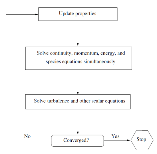
The density-based solver solves the governing equations of continuity, momentum, and (where appropriate) energy and species transport simultaneously (that is, coupled together). Governing equations for additional scalars will be solved afterward and sequentially (that is, segregated from one another and from the coupled set) using the procedure described in General Scalar Transport Equation: Discretization and Solution. Because the governing equations are nonlinear (and coupled), several iterations of the solution loop must be performed before a converged solution is obtained. Each iteration consists of the steps illustrated in Figure 23.2: Overview of the Density-Based Solution Method and outlined below:
Update the fluid properties based on the current solution. (If the calculation has just begun, the fluid properties will be updated based on the initialized solution.)
Solve the continuity, momentum, and (where appropriate) energy and species equations simultaneously.
Where appropriate, solve equations for scalars such as turbulence and radiation using the previously updated values of the other variables.
When interphase coupling is to be included, update the source terms in the appropriate continuous phase equations with a discrete phase trajectory calculation.
Check for convergence of the equation set.
These steps are continued until the convergence criteria are met.
In the density-based solution method, you can solve the coupled system of equations (continuity, momentum, energy and species equations if available) using, either the coupled-explicit formulation or the coupled-implicit formulation. The main distinction between the density-based explicit and implicit formulations is described next.
In the density-based solution methods, the discrete, nonlinear governing equations are linearized to produce a system of equations for the dependent variables in every computational cell. The resultant linear system is then solved to yield an updated flow-field solution.
The manner in which the governing equations are linearized may take an "implicit" or "explicit" form with respect to the dependent variable (or set of variables) of interest. By implicit or explicit we mean the following:
implicit: For a given variable, the unknown value in each cell is computed using a relation that includes both existing and unknown values from neighboring cells. Therefore each unknown will appear in more than one equation in the system, and these equations must be solved simultaneously to give the unknown quantities.
explicit: For a given variable, the unknown value in each cell is computed using a relation that includes only existing values. Therefore each unknown will appear in only one equation in the system and the equations for the unknown value in each cell can be solved one at a time to give the unknown quantities.
In the density-based solution method you have a choice of using either an implicit or explicit linearization of the governing equations. This choice applies only to the coupled set of governing equations. Transport equations for additional scalars are solved segregated from the coupled set (such as turbulence, radiation, and so on). The transport equations are linearized and solved implicitly using the method described in General Scalar Transport Equation: Discretization and Solution. Regardless of whether you choose the implicit or explicit methods, the solution procedure shown in Figure 23.2: Overview of the Density-Based Solution Method is followed.
If you choose the implicit option of the density-based solver,
each equation in the coupled set of governing equations is linearized
implicitly with respect to all dependent variables in the set. This
will result in a system of linear equations with  equations for each cell
in the domain, where
equations for each cell
in the domain, where  is the number of coupled equations in the set. Because
there are
is the number of coupled equations in the set. Because
there are  equations per cell, this is sometimes called a "block"
system of equations.
equations per cell, this is sometimes called a "block"
system of equations.
A point implicit linear equation solver (Incomplete Lower Upper
(ILU) factorization scheme or a symmetric block Gauss-Seidel) is used
in conjunction with an algebraic multigrid (AMG) method to solve the
resultant block system of equations for all  dependent variables in each cell.
For example, linearization of the coupled continuity,
dependent variables in each cell.
For example, linearization of the coupled continuity,  -,
-,  -,
-,  -momentum, and energy equation
set will produce a system of equations in which
-momentum, and energy equation
set will produce a system of equations in which  ,
,  ,
,  ,
,  , and
, and  are the unknowns. Simultaneous
solution of this equation system (using the block AMG solver) yields
at once updated pressure,
are the unknowns. Simultaneous
solution of this equation system (using the block AMG solver) yields
at once updated pressure,  -,
-,  -,
-,  -velocity, and temperature fields.
In summary, the coupled implicit approach solves for all variables
( ,
,  ,
,  ,
,  ,
,  ) in all cells at the same time.
If you choose the explicit option of the density-based solver,
each equation in the coupled set of governing equations is linearized
explicitly. As in the implicit option, this too will result in a system
of equations with  equations for each cell in the domain and likewise,
all dependent variables in the set will be updated at once. However,
this system of equations is explicit in the unknown dependent variables.
For example, the
equations for each cell in the domain and likewise,
all dependent variables in the set will be updated at once. However,
this system of equations is explicit in the unknown dependent variables.
For example, the  -momentum equation is written such that the updated
  velocity is a function of
existing values of the field variables. Because of this, a linear
equation solver is not needed. Instead, the solution is updated using
a multi-stage (Runge-Kutta) solver. Here you have the additional option
of employing a full approximation storage (FAS) multigrid scheme to
accelerate the multi-stage solver.
velocity is a function of
existing values of the field variables. Because of this, a linear
equation solver is not needed. Instead, the solution is updated using
a multi-stage (Runge-Kutta) solver. Here you have the additional option
of employing a full approximation storage (FAS) multigrid scheme to
accelerate the multi-stage solver.
In summary, the density-based explicit approach solves for all
variables ( ,
,  ,
,  ,
,  ,
,  ) one cell at a time.
Note that the FAS multigrid is an optional component of the explicit approach, while the AMG is a required element in both the pressure-based and density-based implicit approaches.