You can refine or coarsen your mesh based on cell registers (Using Cell Registers), named expressions (Named Expressions), or expressions using the Manual Mesh Adaption and/or Automatic Mesh Adaption dialog box, as described in the following steps. For information about adapting overset meshes, see Overset Mesh Adaption.
To set up mesh adaption:
For 3D meshes, you have the choice of refining the cells using either the default polyhedral unstructured mesh adaption (PUMA) method, the 2.5D PUMA method (which is suitable for meshes that are one cell thick), or the hanging node method. For details and limitations on these methods, see Adaption Process in the Theory Guide. To change the adaption method, use the following text command:
mesh→adapt→set→methodBegin the adaption setup by opening the appropriate dialog box:
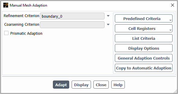
To perform manual adaption, open the Manual Mesh Adaption dialog box.
 Domain → Adapt
→ Manual...
Domain → Adapt
→ Manual...
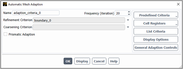
To have the mesh automatically adapted throughout the calculation, open the Automatic Mesh Adaption dialog box.
Domain → Adapt
→ Automatic...
For automatic mesh adaption, enter a Name for the adaption criteria, and specify how frequently Fluent adapts the mesh by setting the Frequency to the number of iterations or time steps that must pass between two consecutive automatic mesh adaptions.
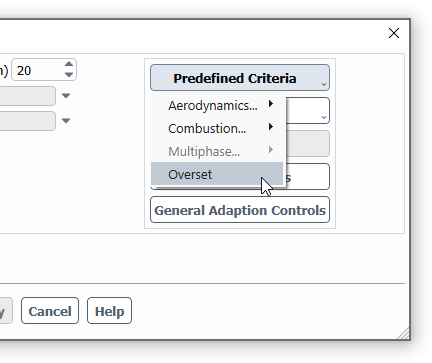
(Optional) You can make a selection from the Predefined Criteria drop-down list to easily set up the adaption with commonly used criteria; this can be done instead of or in combination with the steps that follow. The available criteria are useful for:
meshes that require boundary layer refinement based on a cell's proximity to one or more boundaries
aerodynamic flow simulations that have a shock or significant variations for an error indicator
flows that use a combustion model
flows that use the Volume of Fluid (VOF) multiphase model
overset mesh simulations that are adversely affected by orphans and/or donor-receptor cell size differences
For further details, see Predefined Criteria for Adaption.
(Optional) Create cell registers for the types of cells that you want to adapt by using the drop-down list. For further details, see Using Cell Registers.
Specify the Refinement Criterion you want Fluent to use to determine when the mesh should be refined. You can select an existing cell register or named expression, or provide an expression.
Specify the Coarsening Criterion you want Fluent to use to determine when the mesh should be coarsened. You can select an existing cell register or named expression, or provide an expression.
(Optional) Enable the Prismatic Adaption option if you want the cells to be split anisotropically, that is, only along certain directions. This is typically used with meshes that contain boundary layers (which can be marked using the boundary layer predefined criterion, a boundary register, or a Yplus/Ystar register). The following limitations are associated with this prismatic adaption:
It is for 3D meshes only.
You must use the PUMA adaption method.
Only prismatic cells (that is, hexahedral cells or wedge or polyhedral cells that have the same number of nodes on the top and bottom faces relative to the splitting direction) in layers that are adjacent to a boundary will be refined anisotropically; all other cells will be refined isotropically.
Note: This option corresponds to the
mesh/adapt/set/prismatic-adaption?text command (for manual adaption) and theprismatic?setting that is available when using themesh/adapt/manage-criteria/addtext command (for automatic adaption).When using the Prismatic Adaption option, there are additional global settings that are applied to all adaption criteria, which you can modify if necessary:
By default, the cells that are split anisotropically are divided into two equal halves (that is, with a split ratio of .5). You can change this split ratio using the General Adaption Controls dialog box, as described in a step that follows.
The splitting direction is defined by default as being perpendicular to the boundary zone adjacent to the layers of prismatic cells that are eligible for adaption. Depending on the mesh, some cells may have multiple splitting directions defined by default. You can reduce the number of splitting directions by using the following text command to specify which boundary zone or zones you want used for anisotropic refinement:
mesh→adapt→set→prismatic-boundary-zones
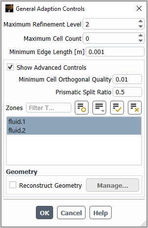
Click the button and define the general adaption settings in the General Adaption Controls dialog box that opens. Note that these settings will be applied to all adaption criteria.
Specify the Maximum Refinement Level, which controls the number of levels of refinement used to split cells during the adaption. A value of zero places no limits on the number of levels. The default of 2 is a good start for most problems. This field essentially keeps Fluent from infinitely refining the mesh. Specifying too large of a value can quickly lead to a very large cell count.
Specify the Maximum Cell Count, which sets an approximate limit to the total cell count of the mesh. Fluent uses this value to determine when to stop marking cells for refinement. A value of zero places no limits on the number of cells. This field is only available with the PUMA adaption method.
Set the Minimum Edge Length. This field restricts the size of the cells that Fluent considers for refinement. Even if a cell is marked for refinement, it will not be refined if (for 3D) its volume is less than the cube of this field or (for 2D) its area is less than the square of this field. The default value of zero places no limits on the size of cells that are refined.
(Optional) Enable Show Advanced Controls to reveal the following advanced controls:
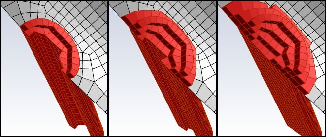
For transient cases, you can specify the number of Additional Refinement Layers that can be refined as part of automatic adaption. Note that the newly marked cells will respect the limits for Maximum Refinement Level and Minimum Edge Length defined in the General Adaption Controls dialog box. When set in the General Adaption Controls dialog box, the Additional Refinement Layers value is a global setting; to customize it for an individual automatic adaption criterion, you can use the
mesh/adapt/manage-criteria/edittext command. The effect of this setting is illustrated in Figure 38.6: Additional Refinement Layers: 1, 2, 3.When you have enabled the Prismatic Adaption option in the Manual Mesh Adaption or Automatic Mesh Adaption dialog box (as described in a previous step), you may want to revise the Prismatic Split Ratio that is applied to the cells, in order to control exactly where the cells are split relative to boundary zones that define the direction. The default value for this ratio is 0.5, and it is defined as follows:

You can specify the Minimum Cell Orthogonal Quality that you would like Fluent to attempt to maintain in the cells that result from adaption. Note that this value is not guaranteed to be maintained, as to do so would negatively affect the solution speed. The worse quality cells will have an orthogonal quality closer to 0 and better quality cells will have an orthogonal quality closer to 1. For more information about cell quality, see Mesh Quality.
Note: The Minimum Cell Orthogonal Quality setting is not available for 2D cases or if the hanging node adaption method is selected.
For cases that have multiple cell zones, you can limit the adaption to a particular cell zone or zones by selecting them in the Zones list. An example of when you might want to do this is when you want to exclude certain cell zones from being adapted, because they already possess sufficient mesh resolution for an accurate result. By default, adaption will be performed in all cell zones.
If you have a coarse mesh on a wall zone that has curved profiles and/or sharp corners, you may want to use geometry-based adaption, so that the new nodes created during adaption are projected onto a specified auxiliary geometry definition. In this way, you can recover finer details of the wall zone shape during refinement. For further details about the concepts involved, see Geometry-Based Adaption in the Theory Guide.
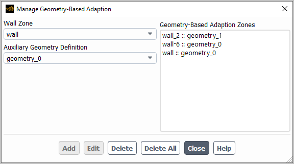
To perform geometry-based adaption using the PUMA adaption method, you must first define one or more auxiliary geometry definitions, as described in Managing Auxiliary Geometry Definitions. Then you can enable the Reconstruct Geometry option under the Show Advanced Controls option, and click the button to open the Manage Geometry-Based Adaption dialog box.
In the Manage Geometry-Based Adaption dialog box, select a Wall Zone and the Auxiliary Geometry Definition to which you want the zone to conform, and click the button (note that you must ensure that the existing nodes on the wall zone already conform to this auxiliary geometry definition). The pair will be listed in the Geometry-Based Adaption Zones list. At any point you can select that Wall Zone again and select a different Auxiliary Geometry Definition and click to edit the definition, or you can select it in the Geometry-Based Adaption Zones list and click to delete it. You can repeat this step with different zones to add additional definitions; note that a zone cannot be paired with more than one geometry definition, but a geometry definition can be paired with multiple zones. Click when your geometry-based adaption is fully set up.
By default, the nodes that move to conform to the geometry definition will only be those on the wall zone surface. If you would like the boundary displacement to also be applied to some degree to the prismatic boundary layers adjacent to the surface, you can use the following text command to edit the relevant geometry-based adaption zone(s) and enter a positive, nonzero value for the
exponent. Lower values for theexponentcause the displacement to propagate further from the surface, and a value of 0 disables such propagation altogether. It is recommended that you start with a value of 0.01 and adjust as needed.mesh→adapt→geometry→manage→editNote: If you want to perform geometry-based adaption when using the hanging node adaption method, you must use the Geometry Based Adaption Dialog Box, as described in Geometry-Based Adaption with the Hanging Node Method.
Click to close the General Adaption Controls dialog box, and continue setting up the Manual Mesh Adaption or Automatic Mesh Adaption dialog box.
(Optional) Click to print the number of cells that Fluent has identified for being refined, coarsened, or both, to the console.
(Optional) Click to open the Display Options - Adaption Dialog Box, which allows you to customize how the cells marked for adaption are displayed.
(Optional) Click to review the cells that are marked for adaption.
For manual adaption, click to adapt the mesh. Note that if at any point you want to switch to using automatic adaption, you can click the to copy the settings to the Automatic Mesh Adaption dialog box.
For automatic adaption:
Click to save the adaption criterion.
Create additional adaption criteria as needed, as described in the previous steps.
Domain → Adapt
→ Automatic...
(Optional) You can specify that one or more of the initial instances of adaption are skipped for a given automatic adaption criterion. This can be done using the following text command:
mesh→adapt→manage-criteria→editAfter entering the name of the criterion to edit, enter
skip-until, followed by a positive, nonzero integer that defines the iteration / time step when automatic adaption is allowed to begin. By default this field is set to1, so that adaption is applied during the first iteration / time step and is never skipped.The following is an example to illustrate how it works: you could set
skip-untilto 40 iterations, and if the frequency is set to 20, adaption will be skipped on the first and twentieth iterations, and will not begin until the fortieth iteration. This is true even if you were to stop the calculation at the thirtieth iteration and then restart (that is, it will skip adaption until the tenth iteration after the restart, because it is based on the iteration count as printed in the console).
Note:The
skip-untilsetting can also be defined when adding a new automatic adaption criterion through themesh/adapt/manage-criteria/addtext command.The
skip-untilsetting is automatically set to2for the Pressure Hessian Indicator, Mach Hessian Indicator, and Combined Hessian Indicator predefined criteria, as typically the calculation of these indicators do not yield useful results in the first iteration / time step. For further details on these criteria, see Aerodynamics Adaption.
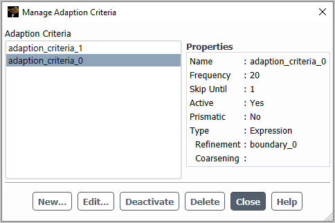
Review your adaption criteria using the Manage Adaption Criteria dialog box.
Domain → Adapt
→ Manage...
If you make a selection from the Adaption Criteria list, information about that criterion is displayed under Properties. You can then: click the button to revise the settings; click if you do not want to use the criterion for the time being (the button will change to so that it can be used later); and click to delete the criterion entirely.
Run your calculation, and your adaption will be automatically applied at regular intervals.
A drop-down list is available in the Manual Mesh Adaption and Automatic Mesh Adaption dialog boxes to increase the ease of setup. It provides a list of commonly used criteria for adapting the mesh; if one is selected, Fluent will generate the necessary cell registers and/or named expressions for refinement and coarsening, and will define the associated settings. Note that your predefined criteria selection may require you to specify certain mandatory settings (such as the Minimum Cell Length Scale), based on the details of your case.
For details, see the following:
You can use predefined criteria to easily adapt the mesh manually for boundary layers, based on a cell's proximity to one or more boundaries. Fluent will automatically generate the necessary cell register for refinement and, where possible, will enable prismatic adaption so that the cells are only split along certain directions.
To use predefined criteria for adapting a boundary layer, perform the following steps:
Read a mesh. If you want prismatic adaption, it must be a 3D mesh that contains prismatic cells adjacent to the relevant boundary zones. Prismatic cells are hexahedral cells or wedge or polyhedral cells that have the same number of nodes on the top and bottom faces relative to the splitting direction.
If you want prismatic adaption, ensure that the PUMA method is selected by using the following text command:
mesh→adapt→set→methodOpen the Manual Mesh Adaption dialog box.
Domain → Adapt
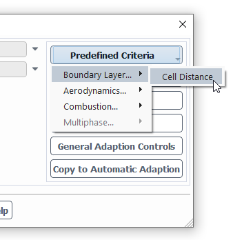
→ Manual... Select Boundary Layer... from the Predefined Criteria drop-down list, and then select Cell Distance from the menu that opens.
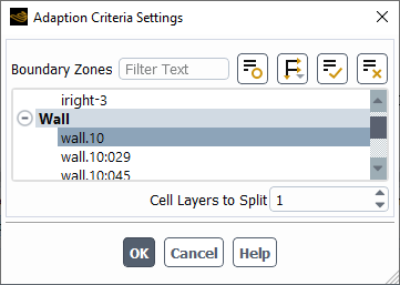
Complete the setup in the Adaption Criteria Settings dialog box that opens. You must select the Boundary Zones where you want adaption, define the number of Cell Layers to Split, and click .
When using the PUMA adaption method, by default the Prismatic Adaption option will be enabled, so that the cells are refined anisotropically where possible; such cells will only be split along the directions that are perpendicular to the zones selected in the Adaption Criteria Settings dialog box. Note that you can control exactly where the cells are split by revising the value for the Prismatic Split Ratio field in the General Adaption Controls dialog box, as described in Refining and Coarsening.
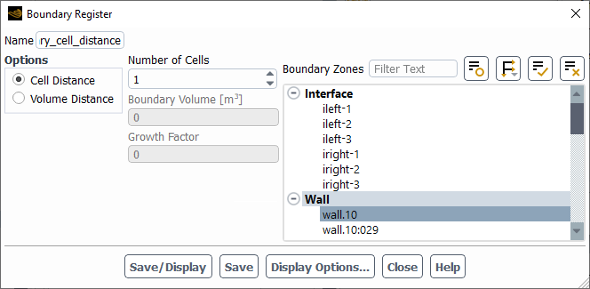
A cell register named boundary_cell_distance is created as part of the predefined criteria and selected in the Refinement Criterion field. Review it in the Boundary Register dialog box to verify that it is appropriate:
 Solution → Cell
Registers → boundary_cell_distance
Solution → Cell
Registers → boundary_cell_distance
 Edit...
 Note that the Boundary Register dialog box allows you to switch to the Volume Distance method when the Cell Distance method is not preferred for your case.
Click in the Manual Mesh Adaption dialog box to perform the adaption.
When simulating aerodynamic flows, you can use predefined criteria to set up the mesh adaption. With this predefined criteria, Fluent will automatically generate the necessary cell registers for refinement and coarsening, based on the gradient of the density (in order to account for shocks), an indicator for error in the pressure calculation (in order to account for significant pressure variations), an error indicator that considers variations in the Mach number, an indicator for error in an observable calculation due to mesh refinement, or an error indicator that considers variations in several flow fields.
To use predefined criteria for adapting a mesh for aerodynamic simulations, perform the following steps:
Set up your aerodynamic simulation, and initialize and/or run the calculation to generate data.
When setting up the mesh adaption for an adjoint observable:
Define the observable to be used for mesh adaption. For details on defining observables see Defining Observables.
Initialize and compute the adjoint solution.
After calculating the adjoint solution, the Goal based error indicator (Raw) field variable can be displayed (under the Sensitivities... category) to identify regions where mesh adaption will have a larger or smaller effect on the observable. High value regions will have a larger effect on the observable and will benefit from cell refinement, whereas low value regions will have a smaller effect on the observable and may benefit from cell coarsening.
Open the Manual Mesh Adaption or Automatic Mesh Adaption dialog box.
Domain → Adapt
→ Manual...
or
Domain → Adapt
→ Automatic...
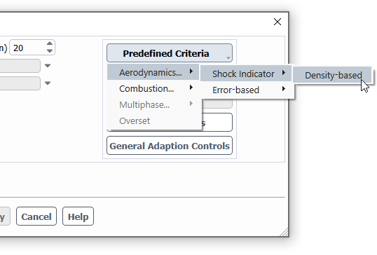
Select Aerodynamics... from the Predefined Criteria drop-down list, and then select one of the following from the menus that open:
Shock Indicator and Density-based
This is useful if you want to adapt the mesh to properly account for shocks, based on the gradient of the density. This criterion is always available if you have selected the Density-Based solver in the General task page, but is only available with the Pressure-Based solver if you have also selected a real-gas or ideal-gas model from the Density drop-down list in the Create/Edit Materials Dialog Box for the fluid.
Error-based and Pressure Hessian Indicator
This is useful if you want to adapt the mesh to properly account for significant pressure variations. It is based on the solution error, as approximated using an indicator that includes the Hessian (the matrix of second derivatives) of the pressure distribution. It targets key areas for adaption in cases with a variety of different scales and flow phenomena: for example, you can capture a shock and wake with different strengths simultaneously, or anisotropic features like errors in stretched prism layer cells. For further details on how the indicator is calculated, see the description of the Hessian approach in Approaches For Deriving Field Values.
Note: This criterion is not recommended for cases with a very smooth solution, as it may target widespread areas and lead to excessive refinement.
Error-based and Mach Hessian Indicator
This is useful if you want to adapt the mesh based on an error indicator that considers variations in the Mach number. This indicator includes the Hessian (the matrix of second derivatives) of the Mach number. It targets adaption for a wider range of Mach number flows compared to the Pressure Hessian Indicator while being based on only a single scalar value for the input field, in contrast to the multiple flow fields used in the Combined Hessian Indicator. For further details on how the indicator is calculated, see the description of the Hessian approach in Approaches For Deriving Field Values.
Note: The Mach Hessian Indicator criterion is only available if the density of the fluid material is defined using the ideal gas law or a real gas model.
Error-based and Combined Hessian Indicator
This is useful if you want to adapt the mesh based on an error indicator that considers variations in several flow fields (pressure, temperature, velocity, density, and turbulence, when each is applicable). This indicator includes the Hessian (the matrix of second derivatives) of these field variables. It is suitable for use across a range of Mach numbers, and can target key areas for adaption in cases with a variety of different scales and flow phenomena. For further details on how the indicator is calculated, see the description of the Hessian approach in Approaches For Deriving Field Values.
Error-based and Goal-Based Error Indicator
This indicator is used to adapt the mesh to reduce the influence of mesh refinement on an observable as part of an adjoint calculation. Selecting Goal-Based Error Indicator will open the Adaption Criteria Settings dialog box, where you can customize the adaption settings for your case. For details on defining these settings see Adaption Criteria Settings Dialog Box.
After setting up the adaption criteria and before computing the flow solution, you can set up solution monitors for the observable and the cell count to observe the change in the observable during mesh adaption and the total cell count, respectively.
Once the necessary adaption and refinement/coarsening criteria have been defined for your case, you can calculate the conventional flow solution to begin the mesh adaption.
Note: Typically the calculation of the Pressure Hessian Indicator, Mach Hessian Indicator, or the Combined Hessian Indicator does not yield useful results immediately after initialization or during the first iteration / time step. For this reason, the
skip-untilsetting is automatically set to2for any automatic adaption that uses these predefined criteria; for further details on theskip-untilsetting, see Refining and Coarsening.For an automatic adaption criterion, by default the cells will be refined at a Frequency based on the criterion:
Density-based:
2time steps /20iterationsPressure Hessian Indicator:
20time steps /20iterationsMach Hessian Indicator:
100time steps /100iterationsCombined Hessian Indicator:
100time steps /100iterationsGoal-Based Error Indicator:
100time steps /20iterations
You can adjust this setting as necessary: for example to allow more convergence between steps to avoid oscillating refinement / coarsening of a region. Note that for the Mach Hessian Indicator or Combined Hessian Indicator criterion, a longer frequency should be used compared to gradient registers, as these indicators are more sensitive to small variations and so may otherwise apply unneeded adaptations due to local fluctuations in the solution.
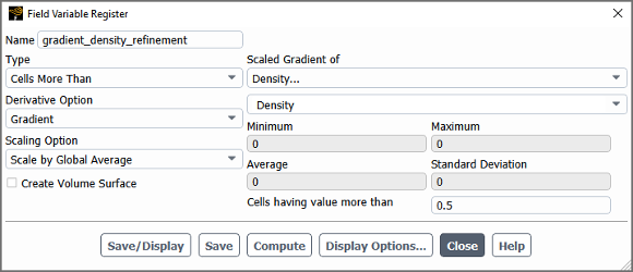
Cell registers are created as part of the predefined criteria. Note their names in the Refinement Criterion and Coarsening Criterion fields or in the console, and review them in the Field Variable Register dialog box to verify that they are appropriate. For example:
Solution → Cell
Registers → gradient_density_refinement
Edit... Note that for the Mach Hessian Indicator or the Combined Hessian Indicator, the resulting cell registers use the Hessian derivative option, which is described in Field Variable. If you change the setup, existing indicators of these types may become invalid and may need to be adjusted or regenerated.
The indicator used in the Pressure Hessian Indicator criterion can be postprocessed by selecting the Pressure Hessian Indicator field variable (under the Derivatives... category). Note that this field variable is scaled by the global average in the cell registers created for the adaption predefined criterion, as it is a relative value.
Predefined criteria is available for adapting the mesh of a combustion simulation, so that the mesh is refined along a progressing flame front using various criteria like temperature, vorticity, species, and DPM concentration (depending on which models are used). There is also an option for refining a spherical spark region prior to a transient run, which after a specified time is then coarsened back to the original mesh. To use this predefined criteria, perform the following steps:
Enable a combustion model.
Setup → Models
→ Species Edit...
Ensure that the energy equation is enabled.
Setup → Models
→ Energy On
Set up your simulation, and initialize and/or run the calculation to generate data.
Open the Manual Mesh Adaption or Automatic Mesh Adaption dialog box.
Domain → Adapt
→ Manual...
or
Domain → Adapt
→ Automatic...
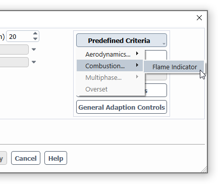
Select Combustion... from the Predefined Criteria drop-down list, and then select Flame Indicator from the menu that opens.
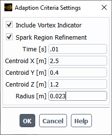
Complete the setup in the Adaption Criteria Settings dialog box that opens:
The Include Vortex Indicator option (which is enabled by default) specifies that the magnitude of vorticity is included as part of the criteria for refinement and coarsening.
Enable the Spark Region Refinement option to refine a temporary spherical spark region at the start of the simulation, which will then be coarsened back to the original mesh. The following settings define the spark region:
Time sets the maximum time during which refinement is applied to the spark region.
The Centroid X, Y, and Z fields set the coordinates for the center of the spark region.
Radius sets the radius of the spherical spark region.
For an automatic adaption criterion, by default the cells will be refined at a Frequency of
2iterations or time steps. You can adjust this setting as necessary.Other adaption settings are defined as part of the predefined criteria. Click the button and review them in the General Adaption Controls dialog box to verify that they are appropriate.
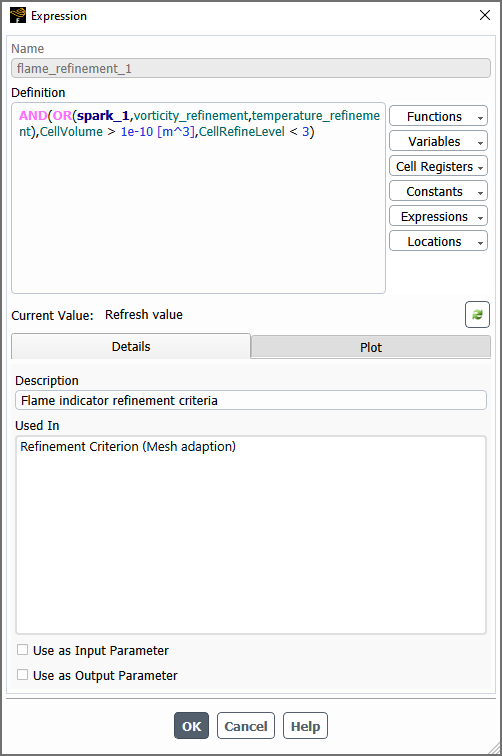
Named expressions are created as part of the predefined criteria. Note their names in the Refinement Criterion and Coarsening Criterion fields or in the console, and review them in the Expression dialog box to verify that they are appropriate. For example:
Setup → Named
Expressions → flame_refinement_1
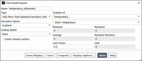
Edit... The named expressions may use cell registers that are also created as part of the predefined criteria. You can review them in the Field Variable Register dialog box. For example:
Solution → Cell
Registers → temperature_refinement
Edit...
When using the Volume of Fluid (VOF) multiphase model (with or without the VOF-to-DPM model transition mechanism), you can use predefined criteria to set up the mesh adaption. With this predefined criteria, Fluent will automatically generate the necessary cell registers (based on field variables) and/or named expressions for refinement and coarsening, based on the volume fraction of the secondary phase.
To use predefined criteria for adapting the mesh of a VOF simulation, perform the following steps:
Enable the Volume of Fluid multiphase model.
Setup → Models
→ Multiphase Volume of
Fluid
Set up your VOF simulation, and initialize and/or run the calculation to generate data.
Open the Manual Mesh Adaption or Automatic Mesh Adaption dialog box.
Domain → Adapt
→ Manual...
or
Domain → Adapt
→ Automatic...
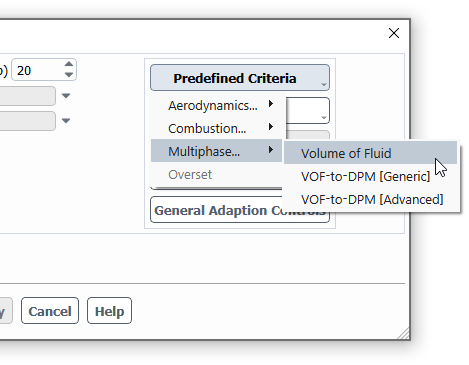
Select Multiphase... from the Predefined Criteria drop-down list, and then select one of the following from the menu that opens:
Volume of Fluid: This is suitable for standard VOF simulations.
VOF-to-DPM [Generic]: This is suitable when using the VOF-to-DPM model transition mechanism; the resulting adaption criterion will be defined by fairly straightforward cell registers.
VOF-to-DPM [Advanced]: This is suitable when using the VOF-to-DPM model transition mechanism; the resulting adaption criterion will be defined by more complex expressions that draw upon cell registers as well as parameters that you will need to define.
An Information dialog box will open to notify you that you must define additional settings or parameters in the refinement / coarsening criterion expression; follow the instructions to complete the setup in the Adaption Criteria Settings dialog box that also opens.
For an automatic adaption criterion, by default the cells will be refined at a Frequency of
2iterations or time steps. You can adjust this setting as necessary.Other adaption settings are defined as part of the predefined criteria. Click the button and review them in the General Adaption Controls dialog box to verify that they are appropriate.
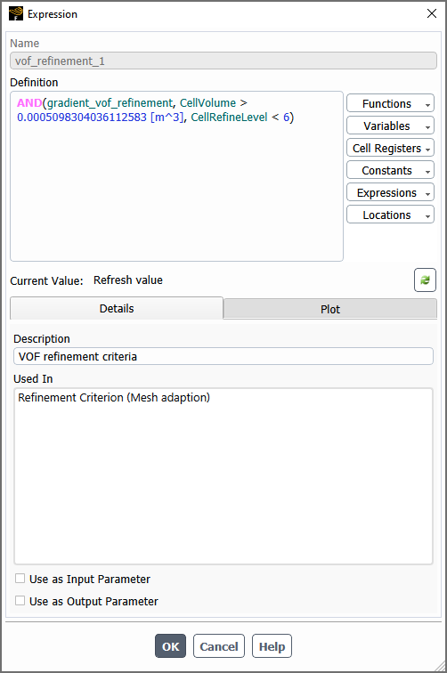
Named expressions and cell registers will be created as part of the predefined criteria. Note their names in the Refinement Criterion and Coarsening Criterion fields or in the console, and review them in the Expressions and Field Variable Register dialog boxes to verify that they are appropriate. For example:
Setup → Named
Expressions → vof_refinement_1
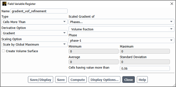
Edit... The previous expression uses the following cell register:
Solution → Cell
Registers → gradient_vof_refinement
Edit...
![The Adaption Criteria Settings Dialog Box for the VOF-to-DPM [Advanced] Criterion](graphics/flu_ug_adapt_crit_set.png)
You can use predefined criteria to easily set up automatic adaption for an overset mesh, with the goal of removing orphan cells, reducing size mismatches between donor and receptor cells, and/or increasing the mesh resolution in gaps as needed (in order to prevent the creation of orphan cells). Typically the overset meshes that benefit from automatic adaption involve moving and dynamic meshes, where it can be difficult to create an initial mesh that meets all of the needs throughout the simulation while also being computationally efficient. Unlike the other predefined criteria, cell registers are not used for the overset predefined criterion, but instead overset-specific adaption tools analyze the initialized overset interface and perform marking and adaption of cells in a single step. Note that by default, 3D prismatic cells that are deemed suitable will be refined anisotropically as part of overset orphan adaption and/or overset gap adaption, in order to reduce the resulting cell count.
To use predefined criteria for automatically adapting an overset mesh, perform the following steps:
Set up your overset mesh simulation, being sure to define an overset interface.
Open the Automatic Mesh Adaption dialog box.
Domain → Adapt
→ Automatic... Select Overset from the Predefined Criteria drop-down list.
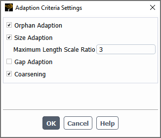
Complete the setup in the Adaption Criteria Settings dialog box that opens:
You can enable the Orphan Adaption option to attempt to remove orphan cells. For details, see Marking for Orphan Adaption.
You can enable the Size Adaption option to reduce size mismatches between donor and receptor cells. For details, see Marking for Size Adaption. As part of this option, you can define the Maximum Length Scale Ratio threshold (
 ) used to determine which cells are marked for adaption based
on donor-receptor cell size differences; this is set to 3 by default.
) used to determine which cells are marked for adaption based
on donor-receptor cell size differences; this is set to 3 by default.You can enable the Gap Adaption option to increase the mesh resolution in gaps as needed (in order to prevent the creation of orphan cells). For details, see Marking for Gap Adaption. As part of this option, you can define the target (minimum) Gap Resolution used when marking cells for gap adaption; this is set to 4 by default.
You can enable the Coarsening option to coarsen the mesh if mesh refinement is no longer needed.
Click to save the settings.
You can review and adjust additional automatic overset adaption settings in the
define/overset-interfaces/adapt/settext command menu, as described in Overset Adaption Controls.