


System Coupling generates coupling output in EnSight file formats, which makes it possible to load results into for high-performance 3D postprocessing. By default, System Coupling automatically produces postprocessing files at initialization, after each restart point, and at the end of the run. These files can be loaded into EnSight for interactive postprocessing, including visualization and animation, of coupled analysis results.
Note: EnSight output will not be created if all interfaces in the analysis contain sides without regions defined. However, results are written for the interface sides containing regions.
Available EnSight results formats:
EnSight Gold Case files (*.case)
EnSight Dynamic Visualization Store (DVS) files (*.dvs)
Note: This documentation assumes that you have already installed and configured EnSight as described in the Necessary Prerequisites section of the Getting Started with Ansys EnSight guide.
For more information, see:
The EnSight-formatted postprocessing files generated by System Coupling are summarized below:
- Command files:
A single command file (*.enc) is written for the coupled analysis according to the type of results being generated for the run (EnSight Gold or EnSight DVS).
It contains all the data for the analysis — that is, it references all the relevant output files, including the case files for all processors used to execute the solution.
Use this file to load coupling results from System Coupling's GUI or CLI or when starting EnSight from the command line.
- EnSight Gold Case files:
An EnSight Gold Case file (Results*.case) is written for each process that System Coupling spawns for the analysis. When multiple processes are used, file names are indexed to ensure uniqueness.
Each Case file contains only the data generated by the associated process.
Use these files after the simulation is complete to open to open coupling results in an existing instance of EnSight.
- Dynamic Visualization Store (DVS) files:
When EnSight's live visualization capabilities are enabled, the Dynamic Visualization Store (DVS) user-defined writer exports the co-simulation's active variables to DVS-formatted files (*.dvs).
- Geometry data files:
Geometry data files have a .geo extension. Geometry results are written for each restart point and at the end of the run.
- Variable data files:
Variable data files have a .dat extension. For each variable, coupling step results are written for each restart point and at the end of the run.
- Multi-step data files:
- Filenames file:
EnSight's Filenames file is named Results.filenames. This file tells EnSight how to complete the filenames.
- Time file:
EnSight's Time file is named Results.time. This file provides the time (in seconds) for transient runs.
For more detailed information on these files, see Ansys EnSight Results Files.
During execution of a coupled analysis, System Coupling generates results files in the Ansys EnSight Gold case file format and writes them to the SyC/Results folder in the co-simulation working directory.
By default, System Coupling automatically produces EnSight results files at analysis initialization, after each restart point, and at the end of the run. The subsequent postprocessing files are generated at the same frequency as restart points, as defined by the OutputControl.Option setting (which itself defaults to generating a single restart point at the end of the coupling run).
For more information on EnSight Gold results, see:
Settings defined under OutputControl.Results control how and when EnSight postprocessing files are auto-generated. Change setting values as described below:
Changing Results-Generation Settings in the GUI
In the GUI's Outline tree under Setup, expand Output Control and click Results.
Edit setting values below in the Properties pane.
Changing Results-Generation Settings in the CLI
In the CLI, change setting values using the method shown in the example below.
>>> DatamodelRoot().OutputControl.Results.Option = 'StepInterval'
>>> DatamodelRoot().OutputControl.Results.OutputFrequency = 2
You can generate EnSight Gold results on-demand from the CLI by running the WriteEnSight() command, providing the name of the file to be generated as an argument.
>>> WriteEnSight(FileName='EnSightResults')
- Retaining existing time step results when restarting a run
When a coupled analysis is restarted, System Coupling reads the contents of the Results folder and removes the following files:
Results files for time steps beyond the initial step of the restarted run
EnSight Command, Case, Filenames, and Time files
To postprocess time steps beyond the step at which the restarted run was opened, ensure that you either back up or rename the Results directory before reopening the case in System Coupling.
- Generating results when a participant does not support restarts
When a coupling participant does not support restarts, EnSight results are generated for the analysis as follows:
If OutputControl.Results.Option is set to the default value of
Program
									Controlled
, then results are generated only at the end of the analysis, regardless of the restart settings specified by OutputControl.Option.If OutputControl.Results.Option is set to a non-default value, then results are generated as specified by the selected value.
Once results are generated for a coupled analysis, there are multiple ways to load them into EnSight for postprocessing. You can load System Coupling's EnSight Gold-formatted results into EnSight either when starting a new instance of EnSight or by opening them in an existing instance of EnSight.
For more information, see:
Note: Ansys recommends loading results into EnSight from System Coupling's GUI or CLI.
To load results in the GUI, use one of the following options:
Right-click the Solution branch and select .
From the Menu Bar, selelct > .
On the Toolbar, click
 .
.
While the results are being opened, a confirmation message is shown on the Command Console tab.
The EnSight GUI opens with the coupling results already loaded.
After the results are loaded, you may close the System Coupling GUI.
In System Coupling's CLI, run the OpenResultsInEnSight() command, as shown below:
>>> OpenResultsInEnSight()
A confirmation message is shown, indicating that the results are being opened. The EnSight GUI opens with the coupling results already loaded.
After the results are loaded, you may close System Coupling's CLI.
When starting EnSight from the command line, you can load System Coupling's EnSight Gold-formatted results by appending command-line arguments to EnSight's executable. When loading results by this method, Ansys recommends that you use the EnSight Command file (Results.enc) generated for the coupled analysis.
To load results when starting EnSight, perform the following steps:
Open a command-line interface for your operating system in the SyC/Results folder for the coupled analysis.
Note: If you open the command-line interface in another folder, you must use EnSight's --cwd command-line argument to set the path of the Results folder as EnSight's working directory. Simply opening the command prompt and specifying the path to the Results.enc file will not work.
Execute the platform-appropriate command, using EnSight's -p command-line argument to specify the name of the EnSight Command file to be played when EnSight is opened, as shown in the examples below.
Windows
"%AWP_ROOT242%\CEI\bin\ensight.bat" -p Results.enc
Linux
$ "$AWP_ROOT242/CEI/bin/ensight" -p Results.enc
The EnSight GUI opens with the coupling results already loaded.
For more information about the -p argument, see Playing a Command File on Startup in the Ansys EnSight How-To Manual.
For information on other EnSight's command-line arguments, see Basic Usage in the Command Line Start-up Options section of the Ansys EnSight How-To Manual.
You can open System Coupling's EnSight Gold-formatted results in an instance of EnSight that is already open. When loading results using this method, Ansys recommends that you use the EnSight Gold Case files (.case) generated for the coupled analysis.
To open results in an existing instance of EnSight, perform the following steps:
Select .
The Open dialog opens.
On the Open dialog:
Ensure that Replace data for current case is selected.
Click to close the dialog.
Use the Look in field to navigate to the SyC/Results folder for the coupled analysis.
Select .
The interface for loading a list of input files is shown below.
Locate and multi-select the Results_<
#>.case files.Note: Ensure that all case files are selected. There is one Case file for each System Coupling process in the coupled analysis.
Click .
The corresponding field is populated with the path to each of the selected files.
Click .
The dialog closes and the results corresponding to the selected Case files are loaded into EnSight.
When co-simulation results are loaded into EnSight, results are populated to the user interface as described in the following sections:
Note: System Coupling does not enforce uniqueness of display names, but for postprocessing, modifies the variable names in the EnSight-formatted results to conform to EnSight naming requirements. These naming modifications are applied only to the EnSight-formatted results. Object display names are unchanged in System Coupling's other outputs.
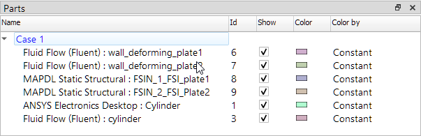
The Parts pane is a table populated with a list of model parts (that is, coupling regions) based on the mesh and associated surfaces defined in the coupled analysis.
Each coupled analysis is loaded into EnSight as a case, named Case and with an index indicating its order in the loading sequence.
Under each Case branch, there is a list of all regions with meshes involved in data transfers.
Each region/part is listed by its display name with a prefix indicating the display name of the corresponding participant and concatenated with additional information, as needed, to ensure that it has a unique name. Parts are named according to the following convention:
<DisplayName> :
<RegionDisplayName_#> |
where:
| "DisplayName" is the participant's DisplayName defined in System Coupling |
| There is a space before and after the colon. |
"#" is an optional index
added when there are duplicate region display names for the same participant
(for example, HeatFlow_1 and
HeatFlow_2). |
Note: These part/region name modifications are applied only to the EnSight-formatted results. Region display names EnSight unchanged in System Coupling's other outputs. When display names are changed for EnSight output, this information is written to the Transcript after the first completed coupling step. For more information, see EnSight Output Display Name Modifications.
For each coupling region, columns show the following information:
Id: Part number or part identifier (as designated in the results file or assigned by EnSight).
Show: When selected, the part is shown in the graphics window (default for all parts on the list).
Color: Color used for the region in the graphics window.
Color by: Variable that determines the part coloring in the graphics window.
You can work with regions as follows:
To change the columns shown in the table, right-click the header row and select Customize.
To change the column values for a region, right-click its row and use the available context options.
To change the attributes of a region, double-click its row and change the desired values in the Edit Attributes for Tagged Model Part dialog that opens.
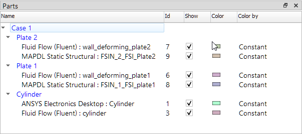
For convenience, you may group regions according to analysis by multi-selecting the involved regions, right-clicking, and selecting Add group/move to group. In the image below, the groups were created in the order the analyses will be addressed in the tutorial.
When results with geometry transformations and/or instancing are written to an EnSight Results file, each reference frame or instance is written as a separate part/region.
Transformation and instancing parts are named according to following convention:
<PartName>_<#>
|
where:
| "PartName" is the name of part/region defined in EnSight (as described in the Parts section) |
| "#" is the number of the reference frame or instance |
Note: These name modifications for transformation and instancing objects are applied only to the EnSight-formatted results. Display names for reference frames and instances are unchanged in System Coupling's other outputs. When display names are changed for EnSight output, this information is written to the Transcript after the first completed coupling step. For more information, see EnSight Output Display Name Modifications.
Note that for a given coupling region, only one orientation and one instance can be shown at a time. For regions involved in multiple coupling interfaces, transformations and instances are displayed as follows:
Transformations:
If a region is involved in multiple coupling interfaces with dissimilar transformations, then it is shown in the GlobalReferenceFrame. To avoid region-orientation disparities in postprocessing output, Ansys recommends that you set up the analysis such that participant regions are transformed into consistent reference frames. For example, you might define the reference frame orientation of each coupling interface such that the geometries are in their actual real-world physical orientation.
Instances:
If different instances are defined for a region that is involved in multiple coupling interfaces, then the reference instance of the region is shown. To avoid region-instancing disparities in postprocessing output, Ansys recommends that you set up the analysis such that the same instance is defined for all occurrences of a given participant region.
The Variables pane is a table populated with variables defined in the coupled analysis data files.
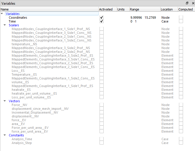
Coordinate and Time variables are activated by default. For each of these variables, columns show values for units (when defined) and range. For mapping statistics variables, the number of source/target values used in the mapping is also shown.
Other variables are grouped by type as Scalars, Vectors, or Constants. Under each of these categories, there is a list of variables relevant to the analysis — that is, variables that are involved in data transfers.
Information on each type of variable is provided in Working with Variables in EnSight.
The Graphics Window shows the regions selected in the Parts list. Operations can be performed on regions shown in the window via the right-click context menus for regions and for the viewport itself.
To toggle between showing and hiding a region in the Graphics Window, select or clear its Show check box in the Parts pane.
System Coupling allows you to view your results dynamically during a co-simulation by sending results (both mesh and solution data) to the EnSight GUI via EnSight's Dynamic Visualization Store (DVS) results files.
Live visualization provides a useful way to verify your co-simulation setup, allowing you to identify areas to be adjusted early in the run, rather than having to wait until the full simulation is complete.
You can also cache your live visualization results so you can open and review them again later.
Note: Note: Currently, the following are not supported for live visualization:
Multiple live visualization objects
Complex numbers
Instances
For more information, see:
To use live visualization during a co-simulation, you must first create a live visualization object.
Note: Currently, System Coupling supports only a single live visualization object. Creation of a second object is blocked in the GUI. Creation of multiple additional objects from the CLI is possible but will result in an error.
- Adding a Live Visualization object in the GUI
In the Outline, right-click the OutputControl branch and select Add Live Visualization.
A Live Visualization branch is added to the Output Control branch, with the new live visualization instance object defined underneath it.
Note: Currently, it is not possible to specify a live visualization object name in the GUI. You can, however, rename existing objects in the CLI.
- Adding a Live Visualization object in the CLI
Add the live visualization object by specifying an object name and an Option setting. Note that you may assign the object any name that conforms to System Coupling's naming conventions.
DatamodelRoot().OutputControl.LiveVisualization['My_FSI_LiveVisualization'].Option = "EveryStep"
By default, the Option setting for a new live visualization object is set to ProgramControlled. Live visualization is disabled with a setting of ProgramControlled or Off, so it simply entails changing this setting to one of the other values.
- Enabling Live Visualization in the GUI
Under Output Control | Live Visualization, click the live visualization object.
Change Option to one of the following values, based on the type of analysis:
LastStep / LastIteration
EveryStep / EveryIteration
StepInterval / IterationInterval (if selected, specify the Output Frequency as usual)
To enable results caching, set Write Results to True.
- Enabling Live Visualization in the CLI
Based on the type of analysis, set Option to a value of LastStep / LastIteration, EveryStep / EveryIteration, or StepInterval / IterationInterval (with a specified OutputFrequency).
DatamodelRoot().OutputControl.LiveVisualization['LiveVisualization1'].Option = LastStep
When enabling live visualization, you can also specify whether the results should be cached for future use. To enable results caching, set the live visualization to write results.
When results caching is enabled, the live visualization results are written to SyC\LV_<objectname>\00000.
- Enabling Results Caching in the GUI
Under Output Control | Live Visualization, click the live visualization object.
Set Write Results to True.
- Enabling Results Caching in the CLI
Set WriteResults to True.
DatamodelRoot().OutputControl.LiveVisualization['LiveVisualization1'].WriteResults = True
When you run a co-simulation case with live visualization enabled, EnSight opens automatically and displays the results as they become available. No other action is necessary on your part.
During the run, the following folders and files are written to the SyC directory:
| Results type | Run type | Folders | Files |
|---|---|---|---|
|
Live results |
Initial run |
LV_<objectname> |
LV_<objectname>.enc LV_<objectname>.dvs |
|
Restarted run |
LV_<objectname>_restart<#> |
LV_<objectname>_restart<#>.enc LV_<objectname>_restart<#>.dvs | |
|
Cached results |
Initial run |
LV_<objectname> |
SyC_<objectname>.dvs |
|
LV_<objectname>\00000 |
metadata.sqlite update_<step/iter #>.h5 | ||
|
Restarted run |
LV_<objectname>_restart<#> |
SyC_<objectname>_restart<#>.dvs | |
|
LV_<objectname>_restart<#>\00000 |
metadata.sqlite update_<step/iter #>.h5 |
To use live visualization for the first time in a new version of EnSight, you must first activate the DVS reader, as follows:
In EnSight, select Edit > Preferences.
In the Preference categories list, select Data.
Under Data preferences:
In the Select below to toggle reader visibility list, locate DVS and ensure that it is turned on—that is, marked with an asterisk ("*").
Click Save to preference file.
Click Close.
The DVS reader is now activated for the current version of EnSight.
Note: You must repeat this process each time you upgrade to a new EnSight version.
There are two ways of viewing live visualization results in EnSight: viewing the live results during the co-simulation and viewing the cached results after the co-simulation has completed.
- Viewing Live Results During the Co-Simulation
When you solve a co-simulation with live visualization enabled, EnSight opens automatically and displays the live results as they become available.
Note: If you have the initial EnSight instance still open when beginning a restarted run, then the restart results open in a second instance of EnSight.
- Viewing Cached Results After the Co-Simulation
To view cached live visualization results for a co-simulation, you must load the results cached in the 00000 folder by opening the SyC_<objectname>.dvs file in a new instance of EnSight.
Important: Before loading cached results, however, make sure that you close the EnSight instance showing the corresponding live results.
To load cached results:
Open a new instance of EnSight and select File > Open.
The Open dialog opens.
Select Advanced interface.
Use the Look in field to navigate to the SyC\LV_<objectname> folder for the coupled analysis.
Locate and select the .dvs file referencing the results you want to load (the file name will begin with "SyC_").
Corresponding information is populated into the Data tab below.
Click Load all parts.
The dialog closes and the results corresponding to the selected Live Visualization file are loaded into EnSight.
To optimize the viewing of System Coupling results, set up the EnSight interface as described in the following sections:
Set up the Graphics Window to provide the most effective display of coupling results, as follows:
Use the menu to turn off the following settings:
Click Perspective to turn off perspective.
Click Highlight selected parts to turn off highlighting.
Turn on the mesh for all regions involved in the analysis.
In the Parts pane, multi-select all the participant regions.
In the Quick Action icon bar above the Graphics Window, click the Part element settings icon (
 ) and
select 3D border, 2D full.
) and
select 3D border, 2D full. In the Tools icon bar at the bottom of the screen, click the Overlay hidden lines icon (
 ).
). The Hidden line overlay color dialog opens.
Select Specify line overlay color.
Click OK to close the dialog.
Set up the viewports so results on each side of the coupling interface are visible at the same time. To do so, perform the following steps:
Split the Graphics Window into two viewports.
Right-click inside the window and select Viewports > 2 vertical.
Note:If you only need to show results on one side of the interface, you may skip this step and keep the single viewport.
Choose the viewport orientation best suited to your model. For example, you would likely use horizontal viewports for a geometry that is elongated along the x axis.
Right-click inside the Graphics Window and select Viewports > Link All.
This links the viewports together so the same view is shown in each.
Limit the display of each participant's interfaces to a single viewport. For each participant:
In the Parts pane, multi-select all regions for that participant.
In the Quick Action icon bar above the Graphics Window, click the Visibility per viewport icon (
 ).
). The Part viewport visibility dialog opens. Both squares are green, indicating that the participant's interfaces are visible in both viewports.
Click a green square.
If you click the square on the left, the right side of the dialog is now black, indicating that the participant's interfaces are now shown only in the left viewport. The opposite occurs if you click the right square.
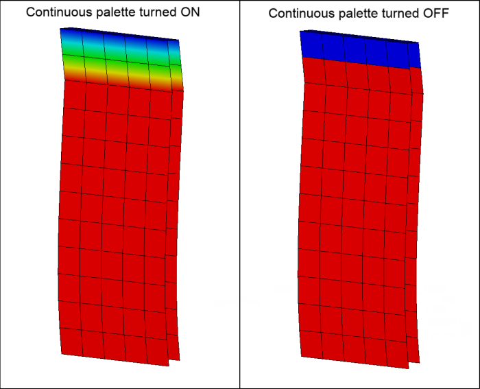
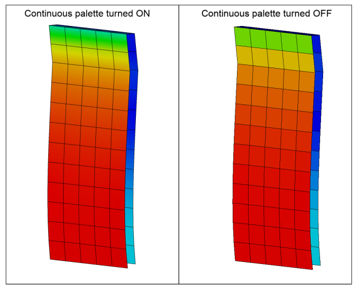
When working with System Coupling results in EnSight, it is generally recommended that you turn off EnSight's continuous palette setting (which is enabled by default).
Coupling participant data may be stored on either nodal or elemental locations. When data are stored on elements, there is a constant value per element. When EnSight's continuous palette setting is enabled, element data are scattered (averaged) to the element's nodes and then presented as though they were nodal data. When the continuous palette setting is disabled, each element is displayed with its constant value, which provides a better representation of how System Coupling has actually mapped the data.
Note: Because nodal data is not scattered, disabling the continuous palette setting has no effect when data is stored on nodes.
To turn off continuous palette coloration, perform the following steps:
Select .
The Preferences dialog opens.
Under Preference categories, select Color Palettes.
Color palette/legend preferences are shown below.
Clear the Use continuous palette for per-element variables check box.
Continuous coloration is now disabled when data on elements are displayed.
For information on working with System Coupling variables in EnSight, review the following sections:
Each variable is listed by its display name, concatenated with additional information, as needed, to ensure that it has a unique name.
Naming conventions vary according to the type of variable.
Variables
<VariableDisplayName_#>__source__<[N|E][S|V]>-->_<[real|imag]>-->
Where:
"
#" is an optional index added when there are duplicate variable display names for the same participant (for example, FluentFluidFlow_1 and FluentFluidFlow_2)The variable display name (with index, when applicable) is followed by two underscores
"source" is an optional indicator added when the source variable has been defined by an expression
"
N" or "E" indicates the variable data Location (Node or Element)"
S" or "V" indicates the variable Quantity Type (Scalar or Vector)" real" or "imag" indicates the Data Type (Real or Imaginary) for complex variable components
Note:
These variable name modifications are applied only to the EnSight-formatted results. Variable display names are unchanged in System Coupling's other outputs. When variable display names are changed for EnSight output, this information is written to the Transcript after the first completed coupling step. For more information, see EnSight Output Display Name Modifications.
System Coupling updates nodal coordinates and related mesh quantities at every coupling iteration after displacement is transferred. To facilitate EnSight postprocessing, System Coupling provides a displacement-since-mesh-import__NV variable. This variable accumulates the displacement calculations since the last mesh import (typically, at the beginning of the analysis or at the last restart) for all incremental displacement variables defined on the coupling interface.
System Coupling creates an area__EV variable for the area vectors of all surface face zones in the analysis. Post-processing this field can be helpful in understanding mapping behavior and to choose the best FaceAlignment setting for advanced situations such as one-sided shells.
Mapping Statistics Variables
Source Side
Used<N |
E>_<interfaceName>_<targetVariableName>
Where "N" or
"E" indicates the
variable data location (Node or Element)
Target Side
Mapped<N |
E>_<interfaceName>_<targetVariableName>
Where "N" or
"E" indicates the
variable data location (Node or Element)
These variables must be activated (loaded into memory) either explicitly by selection of the corresponding Activated check box, or by being called by an operation that requires it.
The EnSight variables used to view data transfer data — whether mapping diagnostics or transferred values — on a given interface side should be determined by the corresponding participant's data location for that data transfer — that is, whether the participant stores data for that quantity type on nodes or elements.
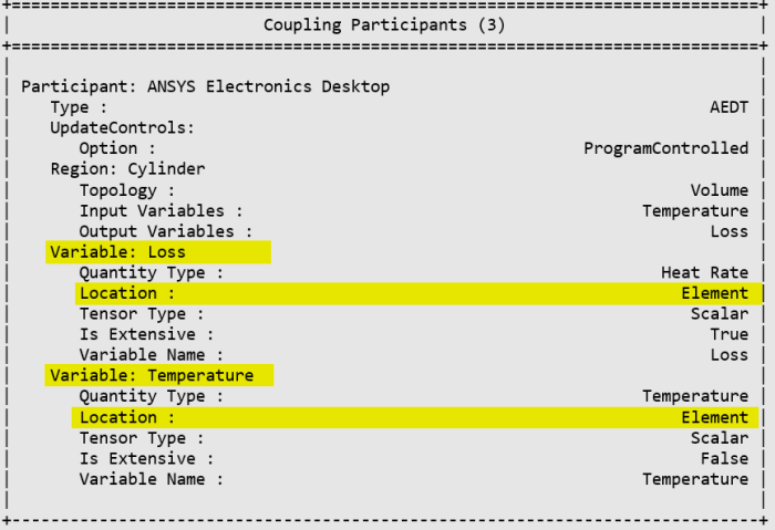
Start out by finding the Location value for each participant variable involved in a data transfer. This information is available in the Coupling Participants section of the Transcript's Summary of Coupling Setup. Data locations are determined by the coupling participants and cannot be changed. Make note of these values, if needed, because you will use this information later to select the variables that match each participant's data location for a given transfer.
The example below shows Maxwell's participant information, with its data transfer variables and corresponding data locations highlighted in yellow.
For data transfers of extensive variables (such as Force or Heat Rate), the amount of the conserved quantity in each mesh element will vary with the sizes of those elements. To facilitate comparison of source and target values on meshes with different element sizes, you should always view the corresponding intensive variables — that is, per-unit-area or per-unit-volume on surface or volume regions, respectively.
In System Coupling analyses, all data transfers are accomplished via mapping, which is the process of calculating data at locations on the target mesh using data from locations on the source mesh. Mapping quality depends upon factors such as the proportion of the target mesh locations that receive data directly from source mesh locations, and the proportion of source mesh locations that are used in those target data calculations. It is important to have high-quality mapping between the source and target meshes on a coupling interface because this will affect the quality of the data transfers.
Note: To assess mapping quality, you should be familiar with System Coupling's mapping process and the types of mapping used in different scenarios. For more detailed information, see System Coupling's Mapping Capabilities.
For more information, see:
Because mapping weights are generated according to mapping type, a given mapping variable covers all data transfers of the specified mapping type that are sent to the specified interface side. For example, if multiple conservative data transfers are sent to the same side of the same interface, the same mapping variable would be applicable to all of them.
Also, a given mapping variable may be applicable to multiple data transfers. For example, a Heat Transfer Coefficient variable and a Convection Reference Temperature variable are transferred as a pair to the same target side on an interface. The same mapping variable will be applicable for these transfers since they both use profile-preserving mapping.
For more information about the mapping type used for various quantities, see Participant Variables and Quantity Types Supported by System Coupling.
To apply a mapping variable, drag it from the Variables pane and drop it on the relevant interface side(s) in the Graphics Window. When evaluating mapping quality, review both the mapped (used) and unmapped (unused) locations on the source and target sides of the interface.
As noted previously, mapping variables indicate how closely the target side of the interface reproduces the source side. Mapping variables are unitless and are displayed in EnSight as follows:
Red (a value of 1) indicates that the location is mapped. Source locations have been successfully mapped to target locations and the source data are being used by the target.
Blue (a value of 0) indicates that the location is not mapped. Source locations have not been successfully mapped to target locations, so the source data are not being used by the target.
To better reflect System Coupling's mapping values, you should configure EnSight as described in Turning Off the Continuous Palette Setting.
To visualize results, you will show variable data on participant regions. One variable may be shown simultaneously on multiple regions, but each region can show only one variable at a time.
To show variable data on a participant region, drag the variable from the Variables pane and drop it onto the corresponding interface side(s) in the Graphics Window.
Note: See the EnSight documentation for other methods applying variables to participant regions.
When the variable is applied:
The variable is activated. In the Variables pane:
The variable name and its parameters are shown as enabled (in black text).
The variable's Activated check is box selected.
The Range parameter is updated with the minimum and maximum values for the range.
Each affected region is colored by the variable.
In the Parts pane, the region's Color by parameter is updated to show the variable name.
In the Graphics Window, variable values are shown on each region and a legend is added to the window.
When comparing data transfer values on both sides of an interface, ensure that plots have palette ranges that are consistent with one another. The goal is to select a range that shows a smooth representation of the full range on both sides of the interface.
Note: Adjusting palette ranges for consistency is effective only for data transfers between like region topologies (that is, transfers between two surface regions or between two volume regions). For data transfers between unlike region topologies, matching ranges will result in poor plots for both models.
In a co-simulation with 2D-3D transfers, it is preferable to plot the transferred quantity using a per-unit-volume variable. For an example, see Visualize Loss Results and Visualize Losses Per-Unit-Volume in the Permanent Magnet Electric Motor Co-Simulation tutorial.
To adjust the palette ranges for data transfer plots, perform the following steps:
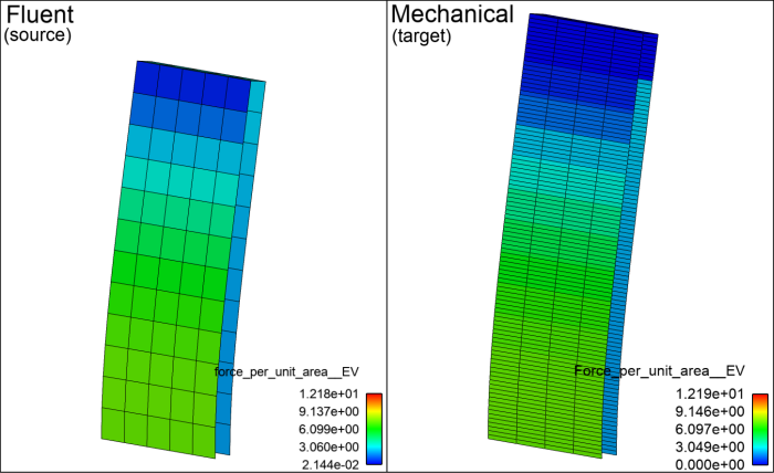
Identify any issues with the representation of the range.
In the example image below, note that the plot palette ranges are dissimilar. Also, neither plot has mesh locations that show values at the upper end of their ranges.
Identify a range that is appropriate for both plots.
Adjust the upper and lower boundary of both ranges as appropriate. For each side of the interface, perform the following steps:
Right-click the palette bar and select Palette > Edit palette.
The Palette Editor dialog opens.
In the field to the right of Range Used, type in the upper range number.
In the field to the left of Range Used, type in the lower range number.
Click Close and then Close again to exit both dialogs.
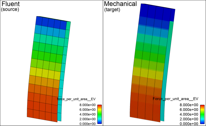
Both plots now share a smooth representation of the full range of values, as shown in the image below.
The following sections provide instructions on EnSight postprocessing tasks that are commonly used in the postprocessing of co-simulation results:
Add a text annotation to a viewport in EnSight.
Right-click inside the viewport and select .
The Create/edit annotation (text) dialog opens.
In the text box, type in the text you to be displayed.
Adjust the size of the text annotation as needed by editing the value of the Size field.
Click Close.
Left-click the annotation to select it.
Holding down the left mouse-button, drag the annotation it to the desired location.
Run a simple animation of solution time steps in EnSight.
In the Solution Time Player (that is, the Time pane), note the value of the Cur field.
The player defaults to using discrete time steps, with the Cur field (the current time step) defaulting to the last time step in the solution.
Set the player back to the first time step setting the field to
0.Leave the player to its default behavior of looping the animation (
 ).
).Run the animation by clicking Play Forward (
 ).
).
Add a simple probe to an animation in EnSight.
In the feature icon bar, click Interactive probe query (
 ).
). The Create/edit probe query dialog opens.
On the Probe create tab:
Under Which variables?, select Coordinates.
Set Query to .
For Probe count, type in the number of probes to be created.
Set the Search fields to Closest node and Pick (use 'p').
The node will be placed on the node closest to the location you select using the 'p' key on your keyboard.
Add the probes, performing the following steps for each:
Left-click the model where you want to add the probe.
Press the 'p' key on your keyboard.
The probes have been added to the model.
Note: On the Create/edit probe query dialog:
To view probe details, click Display results table.
To change the appearance of probes, use the settings on the Display style tab.
To add additional probes, increase the Probe count.
To remove the probes, disable the probe query by setting Query to None.
Add a time annotation to an animation in EnSight.
In the Time pane, click the ellipsis (
 ).
).The Solution time dialog opens.
Note: If the Time pane is not visible, you may display it by right-clicking the Parts pane header bar and selecting Time.
Click Display time annotation.
The Create/edit annotation (text) dialog opens.
Adjust the size of the time annotation as needed by editing the value of the Size field.
Click Close.
Left-click the annotation to select it.
Holding down the left mouse-button, drag the annotation it to the desired location.
Plot nodal displacement as a function of time.
Note: This example uses the results from the Oscillating Plate FSI Co-Simulation with Partial Setup Export from Workbench (CFX-Mechanical) tutorial.
- Create the Function
In the Parts pane, select the fluid region. For this example, select CFX : wall_deforming.
In the Feature Icon bar at the top of the window, click the Calculator icon (
 ).
).The Calculator Tool Box dialog opens.
Click the Build your own functions icon (
 ).
).For Variable name, type in
nodal_position_x.Create an expression.
Under Variable, click Coordinates.
In the calculator, click the [X] button and then the + (addition) button.
Under Variable, click displacement_since_mesh_import__NV.
In the calculator, click the [X] button.
Each of these is added to the Expressions field.
Click the Evaluate for selected parts button.
The nodal_position_x vector quantity is created.
Click Close to exit the dialog.
- Create the Plot
In the Feature Icon bar at the top of the window, click the Query icon (
 ).
).The Create/Edit Query/plot dialog opens.
Under Query Creation, make the following selections:
For Sample, select At node over time.
For Variable 1, select the vector quantity created in the previous step, (N) nodal_position_x.
For Node ID, type in
10.This is the top corner node in the fluid setup.
Click the Create query button.
The plot is added to the Graphics Window.
Click Close to exit the dialog.
You may also create a time annotation and animate the plot, as described in Adding a Time Annotation and Running a Simple Animation of Solution Time Steps, respectively.
Add force vector arrows to an animation.
Note: This example uses the results from the Reed Valve FSI Co-Simulation with Partial Setup Export from Workbench (Fluent-Mechanical) tutorial.
In the Parts pane:
Ensure that the appropriate force per-unit variable is applied to the region to which force is being applied.
In the Reed Valve tutorial example, the Force_per_unit_area__EV variable is applied to Transient Structural : System Coupling Region.
Select that region.
In the Feature Icon bar at the top of the window, click the Vector Arrows icon (
 ).
). The Create Vector Arrows using default attributes dialog opens.
In the blank field near the top of the dialog, you may name the new part to be created. Type in
Force Per-Unit-Area Vector Arrows.Confirm that Variable to is set to the force per-unit vector variable — in this case, (E) Force_per_unit_area__EV.
Optionally, you may wish to adjust the display of the arrows. To do so, ensure that the Advanced check box is enabled and then edit the display parameters as needed. For this example:
Under Creation, for Scale factor type in
2.0000e-07.Under Arrow Tip, leave Size set to Proportional and type in
1.5000e-01.
Click the button.
A Force Per-Unit-Area Vector Arrows entry is added to the Parts pane.
Click Close to exit the dialog.
You can also animate the plot, as described in Running a Simple Animation of Solution Time Steps. The arrow shows the vector of the forces applied to the body.