


During the execution of a coupled analysis, System Coupling generates convergence diagnostic data and plots it on the System Coupling GUI's Chart tab. Charts are available in step, iteration, and simulation-time formats, with the step-based charts shown by default. Additionally, the convergence diagnostics data can be written to a .csv file for analyses run either in System Coupling's GUI or in its CLI.
Diagnostic data are updated dynamically in both the charted and .csv output formats, so both can be used to monitor convergence as the coupling run progresses and or to review the final set of convergence data after the run completes (or is stopped).
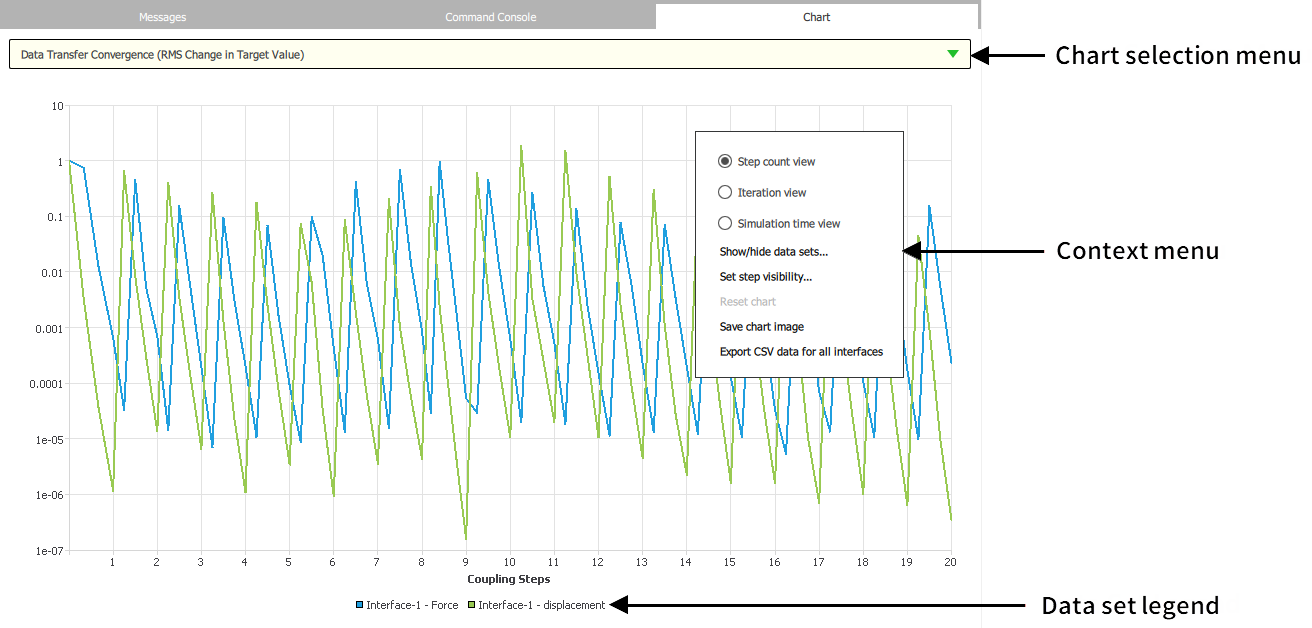
By right-clicking anywhere on the tab, you can access a context menu with options for performing various charting operations.
After a restart, System Coupling resumes updating the same plot lines on existing charts, unless significant changes have been made to the data model (for example, changes to interfaces or data transfers, changed setting values). When there are data model changes, System Coupling generates new charts, starting with the first iteration of the restarted run.
When System Coupling opens or connects to a coupled analysis:
If the coupled analysis was accessed by switching to a different working directory, existing charting data from the previous working directory is removed.
Charts resume at the current solution state and show the history of each data set.
For more information, see:
The System Coupling GUI's Chart tab is shown by default when a solution begins — regardless of whether it is the initial run, a restarted run, or a reconnected run — and relevant data becomes available.
Only one chart can be viewed at a time, and the Convergence Diagnostics chart is shown by default until you change the chart selection.
The following core functionality is available for all charts:
- Active chart selection
The chart-selection drop-down menu at the top of the tab allows you to select a chart from among the charts generated for the simulation. The name selection also serves at the title for the active chart.
- Step, Iteration, and Simulation Time chart views
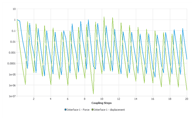
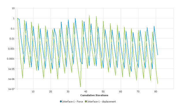
All charts can be viewed in both a step-based and an iteration-based format. Transient charts may also be viewed in a simulation-time format. The step-based chart is shown by default, but you can switch between views using the chart view context menu options.
Steps, iterations, and simulation time are plotted dynamically along the X axis as charting data are generated, as follows:
Labels are shown as simple powers of 10, with the number of labels adjusting according to the extent of the axis.
Steps are plotted with equal spacing.
Iterations are distributed equally within the parent step. With the addition of each new iteration, all existing iterations within the current step are redrawn.
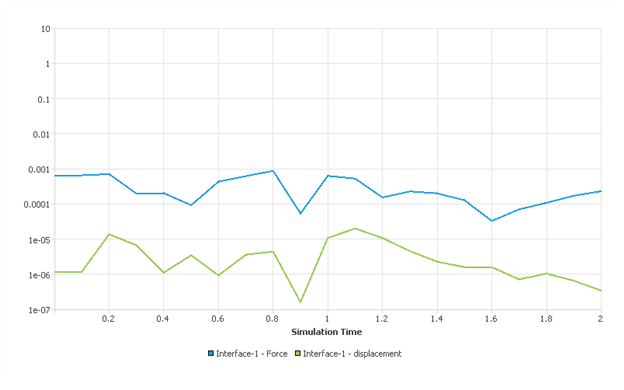
Simulation time is plotted at intervals consistent with whether the steps are of constant or non-constant duration. For the step that is in progress, the value of the most recently available iteration is shown as the current end time. For each completed step, the value for the final iteration of the step is shown as the step end time.
By default, charts show all steps/iterations or the full duration of the simulation. You can specify the number of steps/iterations or time interval to be shown using the visibility context menu options.
- Data set plot lines
Relevant data are plotted on an auto-scaled XY line graph, with a separate line for each individual data set. A legend at the bottom of the tab indicates the name of each data set and the color of the corresponding plot line.
All data sets are selected (that is, all plot lines are shown) by default, but you can show or hide individual data sets using the Show/hide data sets context menu option.
- X-axis chart controls
- Zoom:
Zoom controls allow you to zoom in on the X axis. Dynamic updates pause while the zoom function is active.
To zoom in, click anywhere inside the tab, then either use the mouse wheel or hold down the Ctrl key and use the plus and minus keys (+ and – ) to adjust the zoom level.
To reset the zoom level and resume chart updates, select the Reset chart option from the context menu.
- Pan:
Pan controls are available when the zoom function is active and/or when you have specified the number of steps or iterations to be shown. Dynamic updates pause when the panning function is used.
To pan, click anywhere inside the tab, then either hold down the left mouse key and drag the mouse or use the or the left/right arrow keys to move along the X axis.
To reset the pan location and resume chart updates, select the Reset chart option from the context menu.
- Charting output
Coupling interface charting data can be output to .csv files, either automatically or on-demand. For more information, see Writing Charting Diagnostics to CSV Files.
An image of the active chart can be exported as a .png file using the Save chart image context menu option.
By right-clicking anywhere on the Chart tab, you can access a context menu with options for performing various chart operations. The table below provides details on each available option.
Table 25: Chart context menu options
| Option | Description |
|---|---|
|
Step count view Iteration view Simulation time view
|
These options allow you to select a chart view based on steps, iteration, or simulation time. The step-based view is shown by default. Once specified, the chart view setting persists for the duration of the System Coupling session or until a different view is selected. |
|
Show/hide data sets |
Controls the visibility of the plot lines for individual data sets. By default, all data-set plot lines are shown. When selected, opens a dialog that allows you to select/deselect generated data sets data sets to show/hide their plot lines in the chart. Once specified, data set visibility settings persist for the duration of the System Coupling session or until a different option is selected. |
|
Set step visibility Set iteration visibility Set time interval to show |
Each option is available when the corresponding chart view is selected. Controls the number of steps, the number of iterations, or the time interval that is shown on the displayed charts. Selecting an option opens a dialog with corresponding options. For step-based or iteration-based charts, the following options are available:
For simulation time-based charts, the following options are available:
Once specified, step/iteration/time visibility settings persist for the duration of the System Coupling session or until a different option is selected. |
|
Reset chart |
Available when zoom and/or pan functionality is active. Resets the chart back to its original zoom level and/or pan location and allows chart updates to resume. |
|
Save chart image |
Saves the active chart as a .png file. When selected, opens a Save chart image dialog that allows you to specify a location and a file name for the image. |
|
Export CSV data for all interfaces |
Exports charting convergence diagnostics for all coupling interfaces to .csv files. For more information, see Writing CSV Charting Output On Demand. |
When a solution begins, System Coupling generates a single Convergence Diagnostics chart for the analysis and shows it by default on the Chart tab. This chart includes the convergence data for all data transfers across all interfaces in the analysis.
On this chart, System Coupling plots all the convergence diagnostics — that is, normalized differences per coupling iteration for coupling participants, coupling interfaces, and data transfers — on an XY graph with logarithmic scaling of the Y axis. Each diagnostic is a separate data set with its own line on the chart. At the end of each iteration, the updated value for each diagnostic is added as a new data point.
On the legend, the data sets are identified by interface and data transfer name. The axes of the graph are defined as follows:
Y Axis: End-of-iteration values for each diagnostic.
X Axis: Steps/cumulative iterations/time intervals for the simulation.
System Coupling generates one or more Data Transfer Quantity Diagnostics charts for the analysis. One chart is generated for each data quantity type, and it includes data for all transfers of that quantity across all coupling interfaces in the analysis.
On this chart, System Coupling plots data transfer quantity diagnostics — that is, the Sum for transfers of extensive variables and an area or volume Weighted Average for transfers of intensive quantities — on an XY graph with linear scaling of the Y axis. Each transfer of the given quantity is a separate data set with its own line on the chart. At the end of each iteration, the updated diagnostic value is added as a new data point.
On the legend, each data set is identified by the name of the corresponding data transfer.
The axes of the graph are defined as follows:
Y Axis: End-of-iteration diagnostic values for each data transfer.
X Axis: Steps/cumulative iterations/time intervals for the simulation.
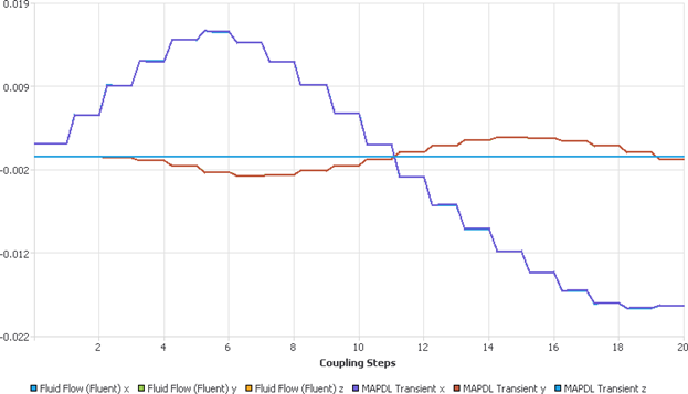
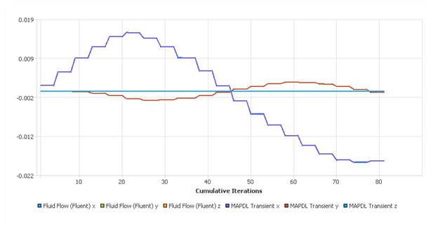
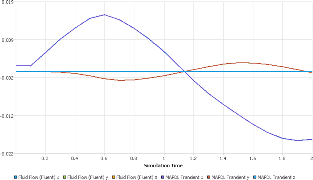
Figure 20: Simulation Time-based Data Transfer Quantity Diagnostic chart showing the Weighted Average
System Coupling can write its charting convergence diagnostics to .csv files, both dynamically as the solution executes and on-demand for data that has already been generated.
For more information, see the following sections:
You can configure System Coupling to write convergence charting data to a .csv file as the analysis is executed. This capability is controlled by the Output Control | Generate CSV Chart Output data model setting.
To enable the generation of .csv output during execution, you can use either of the following methods:
- Enabling Dynamic CSV Charting Output in the GUI
In the Outline tree under Solution, click Output Control and set the Generate CSV Chart Output setting to True.
- Enabling Dynamic CSV Charting Output in the CLI
In the data model, set the OutputControl.GenerateCSVChartOutput setting to
True, as shown below:>>> DatamodelRoot().OutputControl.GenerateCSVChartOutput = True
When the solution starts, System Coupling writes charting data to .csv files
generated in its SyC coupling output directory. One file is
created per interface, with each named according to the convention
<InterfaceName>.csv,
where "InterfaceName" is the
internal name of the interface object in the data model (that is, not the display
name shown in the GUI).
As the solution progresses, each file is updated with its interface's convergence and transfer data for each iteration.
If .csv charting output is enabled, as described in Generating Dynamic CSV Charting Output During the Solution, you can request that all existing convergence charting data for a completed solution are written to a .csv file.
To request on-demand .csv charting output, you can use either of the following methods:
- Requesting CSV Charting Output in the GUI
Right-click anywhere on the Chart tab and select the Export CSV data for all interfaces context option.
- Requesting CSV Charting Output in the CLI
Run the WriteCsvChartFiles() command, as shown below:
>> WriteCsvChartFiles()
When the operation is executed, existing charting data are written to
.csv files in the SyC folder of
System Coupling's working directory. One file is created per interface, with each named
according to the convention
<InterfaceName>.csv, where
"InterfaceName" is the
internal name of the interface object in the data model (that is, not the display
name shown in the GUI).
Note: Files generated will overwrite any .csv charting files that already exist, including any that were written during the execution of the solution.