3.7.2. Spatially Averaged and Spray Panel

Use this panel to control the output of spatially averaged solutions and spray data from the simulation model. Check the Spatially Averaged and Spray box to activate the options. The options are the same as those described for Spatially Resolved data in the previous section, except for the user-defined frequency. The spatially averaged solutions are written as comma-separated-value (.csv) files. Since the spatially averaged data takes up much less space in the solution file, it is not necessary to limit the frequency to the extent that is necessary for the spatially resolved data.

Note: The parameters reported in dynamic.csv, flame.csv, flow_into_cylinder.csv, flow_into_primary_region.csv, mass/molefraction.csv, particle.csv, particle_size_distribution.csv, speciesmass.csv, thermo.csv and two_phase.csv are only for the in-cylinder region (or a primary region, for non-engine cases). If a cylinder/primary region has Sub-Chamber-typed region(s) connected to it, the spatial averaging considers the Sub-Chamber region(s) as part of the cylinder/primary region.

In the Spatially Averaged Species sub-panel, select which gas species data will be saved in the output files. Move species from the Choices list to the Selection list to include them as a Spatially Averaged Species. You can type into the Filter box to limit the species presented in the Choices list. Three .csv files dedicated to species data output. Speciesmass.csv, massfraction.csv, and molefraction.csv include the data of species mass, mass fraction and mole fraction, respectively. If the simulation type is Eulerian two-phase flow (Gas-Phase and Eulerian Two-Phase Flow Simulations), all the liquid species' data will be saved in these solution files.

As for the spatially averaged solution variables and spray variables, Table 3.6: Spatially averaged variables that are always output to the .csv files summarizes the variables’ names, their output files, and their descriptions.

Table 3.6: Spatially averaged variables that are always output to the .csv files

Variable	Output File^[a]	Description
Center of Mass-x	D	The x coordinate of the center of mass in the cylinder. where is the fluid mass contained in a momentum control volume surrounding vertex are the coordinates of vertex . Unit: cm.
Center of Mass-y	D	The y coordinate of the center of mass in the cylinder. Unit: cm.
Center of Mass-z	D	The z coordinate of the center of mass in the cylinder. Unit: cm.
Total angular momentum-x	D	Total angular momentum of the in-cylinder flow in the x direction, relative to the instantaneous mass center in the cylinder. where is the fluid mass contained in a momentum control volume surrounding vertex are the coordinates of vertex are the velocities of vertex , and are the coordinates of the instantaneous charge mass center of the cylinder region. Unit: g-cm²/s.
Total angular momentum-y	D	Similar to Total angular momentum-x, but for the angular momentum in the y direction. Unit: g-cm²/s.
Total angular momentum-z	D	Similar to Total angular momentum-x, but for the angular momentum in the z direction. Unit: g-cm²/s.
Total angular momentum	D	Root mean square of the x-, y-, z-angular momentum. Unit: g-cm² /s.
Tumble ratio-x	D	The ratio of the angular velocity of the in-cylinder flow about the x axis to engine rotating velocity. where is the angular momentum of the in-cylinder mass about the x-axis, is the angular velocity of engine crank, and is the corresponding moment of inertia, defined as: where is the index of the CFD vertices contained in the in-cylinder domain, is the fluid mass contained in a momentum control volume surrounding vertex are the coordinates of vertex , and are the coordinates of the instantaneous charge mass center of the in-cylinder region. Unit: dimensionless.
Tumble ratio-y	D	Similar to Tumble ratio-x, but for the angular velocity in the y direction. where L _y is the angular momentum of the in-cylinder mass about the x-axis, is the angular velocity of engine crank, and I _y is the corresponding moment of inertia, defined as: where is the index of the CFD vertices contained in the d domain, is the fluid mass contained in a momentum control volume surrounding vertex are the coordinates of vertex , are the coordinates of the instantaneous charge mass center of the in-cylinder region. Unit: dimensionless.
Swirl ratio	D	Similar to Tumble ratio-x, but for the angular velocity in the z direction. where is the angular momentum of the in-cylinder mass about the z-axis, is the angular velocity of engine crank, and is the corresponding moment of inertia, defined as: Note that this swirl ratio definition assumes that the axis of the cylinder aligns with the z-axis. Unit: dimensionless.
Total kinetic energy	D	Total kinetic energy of the in-cylinder gas. Unit: g-cm² /s².
Turbulent kinetic energy	D	Mass-averaged turbulent kinetic energy. Unit: cm² /s².
Dissipation rate of TKE	D	Mass-averaged dissipation rate of turbulent kinetic energy. Unit: cm² /s³.
Turbulence velocity	D	Mass averaged turbulent velocity, defined as Where TKE is turbulent kinetic energy. Unit: cm/s.
Integral length scale	D	Mass-averaged turbulence integral length scale. Unit: cm.
Turbulence viscosity	D	Mass-averaged turbulent contribution to the effective kinematic viscosity. The value in each cell is calculated as . Unit: cm² /s.
EffectiveThermal Conductivity	D	Mass-averaged effective (laminar + turbulent) thermal conductivity of the gas phase. Unit: erg/cm-s-K.
Pressure	T	Volume-averaged static pressure. Unit: MPa
Temperature	T	Mass-averaged temperature. Unit: K.
Max Temperature	T	Maximum temperature in the cylinder. Unit: K.
Chemical heat release rate	T	Pure chemical heat release rate in the cylinder or in region 1, calculated directly based on chemical heat release in the cells. Unit: J/deg for engine cases, J/s for non-engine cases.
Accumulated chemical heat release	T	Accumulated chemical heat release rate in the cylinder or in region 1. Unit: J.
Wall heat transfer rate	T	Rate of wall heat transfer through the wall of cylinder or region 1. The heat transfer includes both convective and radiative heat transfer, if applicable. Unit: J/deg for engine cases, J/s for non-engine cases.
Accumulated wall heat transfer	T	Accumulated wall heat transfer loss through the wall of cylinder or region 1. The heat loss includes both convective and radiative heat loss, if applicable. Unit: J.
Apparent heat release rate	T	The difference between chemical heat release rate and wall heat transfer loss rate. Unit: J/deg for engine cases, J/s for non-engine cases. ^[b]
Accumulated apparent heat release	T	Accumulated apparent heat release rate. Unit: J.
Apparent heat release from PV-ConGamma	T	This heat release rate is based on the in-cylinder averaged pressure and volume time/crank angle profiles, assuming a constant gamma (1.35), and is calculated as follows, where dt may also be dCA in engine cases ( t is time, CA is crank angle): Numerically, the gradient terms at time n are calculated using values at time n and n -1, for example, . Unit: J/deg for engine cases and J/s for non-engine cases.
Accumulated apparent heat release from PV-ConGamma	T	Accumulated apparent heat release amount derived from the in-cylinder pressure-volume curve, assuming a constant gamma (1.35). Unit: J.
Apparent heat release from PV-VarGamma	T	This heat release rate is based on the in-cylinder averaged pressure and volume time/crank angle profiles, using variable gamma values, where gamma is the specific heat ratio () of the in-cylinder mixture. The heat-release rate is calculated as: ...where may also be in engine cases ( is time, is crank angle). Unit: J/deg for engine cases and J/s for non-engine cases.
Accumulated apparent heat release from PV-VarGamma	T	Accumulated apparent heat release amount derived from the in-cylinder pressure-volume curve, using variable gamma values. Unit: J.
HeatCapacityConstV	T	Heat capacity of gas-phase mixture at constant volume. Unit: J/Kg-K.
HeatCapacityConstP	T	Heat capacity of gas-phase mixture at constant pressure. Unit: J/Kg-K.
Enthalpy	T	Specific enthalpy of gas-phase mixture. Unit: J/Kg.
In-cylinder mass	T	Total mass of the gas in the cylinder. Unit: g.
In-cylinder volume	T	Total volume of the gas in the cylinder. Unit: cm³.
Region mass	T	Total mass of the gas in a primary region (for non-engine cases). Unit: g.
Region volume	T	Total volume of the gas in a primary region (for non-engine cases). Unit: cm³.
Total volume	T	Total volume of the gas in the whole computational domain. Unit: cm³.
In-cylinder (or Region) averaged equivalence ratio	T	Equivalence ratio calculated using the averaged species mass fractions in a cylinder or primary region, defined as the ratio of oxygen needed to convert carbon and hydrogen to CO₂ and H₂O to the oxygen available in the mixture. Where [C], [H], and [O] are the sum concentrations of carbon, hydrogen, and oxygen atoms in the mixture, respectively: This definition of equivalence ratio is essentially an element ratio that considers all the species in the mixture. It measures the equivalence ratio of a mixture in its unburned state. Using this definition, a mixture’s equivalence ratio remains invariant as it changes from unburned to completely combusted in the combustion process.
In-cylinder (or Region) averaged residual fraction	T	The averaged residual fraction is the mass fraction of the residual mixture in a cylinder or primary region. The residual fraction is estimated by using the equivalence ratio calculated in the row above and the spatially averaged mixture composition as inputs. It also assumes that the fuel is completely converted to combustion product. Specifically, the residual gas includes CO₂, H₂O as well as N₂ needed to generate CO₂ and H₂O through complete combustion. For lean mixtures, the residual also includes excess O₂, subject to its availability in the mixture.
In-cylinder (or Region) averaged progress equivalence ratio	T	The progress equivalence ratio is calculated as: where [C], [H], and [O] are the sum concentrations of carbon, hydrogen, and oxygen atoms in species excluding CO₂, H₂O, and O₂, and [O] from O₂ is the concentration of oxygen atoms from O₂. Using this variation definition, the φ value varies as a combustible mixture changes from its unburned state to completely burned state in the combustion process.
In-cylinder (or Region) averaged progress residual fraction	T	The "progress" residual fraction is calculated using the same assumption as the regular residual fraction described above, but it uses the "progress" equivalence ratio when estimating the N₂ needed to generate the combustion product and the excess O₂ for lean mixtures.
CO	T	Total mass of CO normalized by total fuel mass in the cylinder (for engine cases) or region 1 (for non-engine cases). Unit: g/kg-fuel.
NO	T	Total mass of NO normalized by total fuel mass in the cylinder (for engine cases) or region 1 (for non-engine cases). Unit: g/kg fuel.
NO2	T	Total mass of NO2 normalized by total fuel mass in the cylinder (for engine cases) or region 1 (for non-engine cases). Unit: g/kg fuel.
EINOx	T	Emission index (EI) of NO_x species. In this NOx definition, NO is first converted to NO₂ and then the mass of the converted NO₂ is summed up with the actual NO₂. This parameter is normalized by the total mass of fuel. Unit: g/kg-fuel.
Soot	T	Total mass of soot species normalized by total fuel mass in the cylinder (for engine cases) or region 1 (for non-engine cases). Unit: g/kg fuel.
Unburnt Hydrocarbon	T	Total mass of unburned hydrocarbon (UHC) species normalized by total fuel mass in the cylinder (for engine cases) or region 1 (for non-engine cases). The hydrocarbon species include species that contain both C and H atoms, and no other atoms. Unit: g/kg-fuel.
C1 Unburnt Hydrocarbon	T	ppm of unburned hydrocarbon converted to C1 level. Unit: ppm.
Volatile Organic Compound	T	The volatile organic compound species include species that contain both C and H atoms, and the species may contain other atoms, such as oxygen (O) or nitrogen (N).
C1 Volatile Organic Compound	T	ppm of volatile organic compound converted to C1 level. Unit: ppm.
Average molecular weight	T	Average molecular weight of the gas mixture in the cylinder (for engine cases) or region 1 (for non-engine cases).
Compressibility factor	T	In-cylinder averaged compressibility factor, calculated by , where is static pressure, is density, is the gas constant, and is temperature. For an ideal gas, the compressibility factor is unity.
Number of chemically active cells	C	Number of computational cells in which detailed chemistry is being solved.
Number of clusters in DCC	C	Number of clusters created by the Dynamic Cell Clustering method.
Average number of active species in DAC	C	Averaged number of active species obtained from the Dynamic Adaptive Chemistry method.
Min numbers of active species in DAC	C	Minimum number of active species obtained from the Dynamic Adaptive Chemistry method among all the cells.
Max number of active species in DAC	C	Maximum number of active species obtained from the Dynamic Adaptive Chemistry method among all the cells.
Average number of active reactions in DAC	C	Averaged number of active reactions obtained from the Dynamic Adaptive Chemistry method.
Min numbers of active reactions in DAC	C	Minimum number of active reactions obtained from the Dynamic Adaptive Chemistry method among all the cells.
Max number of active reactions in DAC	C	Maximum number of active reactions obtained from the Dynamic Adaptive Chemistry method among all the cells.
Number of convergence failures	C	Number of convergence failures encountered when solving chemistry in CFD cells or DCC clusters.
Number of transported species	C	Number of species being solved in flow transport. When chemistry is inactive and species lumping has been applied, only a subset of species participates in flow transport.
Only activated with the Spark Ignition model
Burnt Density	F	Density of the burnt gas mixture when the flame propagates. Unit: g/cm³.
Unburnt Density	F	Density of the unburnt gas mixture when the flame propagates. Unit: g/cm³.
S_plasma	F	Averaged plasma velocity of the particles used to track spark-ignition kernel flames. Unit: cm/s.
S_laminar	F	Averaged laminar flame speed of all the cells containing the flame front surface. Unit: cm/s.
S_turb	F	Averaged turbulent flame speed of all the cells containing the flame front surface. Unit: cm/s.
F_stretch	F	Averaged flame stretch factor of all the cells containing the flame front surface. The stretch factor is part of the turbulent flame speed correlation and it accounts for the stretching effect of curvature and turbulence on flame propagation speed. Unit: dimensionless.
R_kernel	F	Radius of the spark ignition kernel flame. Unit: cm.
Number_of_flame_cells	F	Number of cells that contain the flame front surface.
Chem_heat_release_rate_end_gas	F	Chemical heat release rate in the end gas zone. Unit: J/deg for crank-angle-based simulation and J/s for time-based simulation.
Chem_heat_release_rate_flame_front	F	Chemical heat release rate in the end gas zone. Unit: J/deg for crank-angle-based simulation and J/s for time-based simulation.
Chem_heat_release_rate_post_flame	F	Chemical heat release rate in the post flame zone. Unit: J/deg for crank-angle-based simulation and J/s for time-based simulation.
Accum_chem_heat_release_rate_end_gas	F	Accumulated chemical heat release in the end gas zone. Unit: J.
Accum_chem_heat_release_flame_front	F	Accumulated chemical heat release in the flame front zone. Unit: J.
Accum_chem_heat_release_post_flame	F	Accumulated chemical heat release in the post flame zone. Unit: J.
Only activated with the Spray model
Injected mass by injector N	S	Accumulated injected fuel mass at specific time or crank angle from injector N. Unit: g.
Total injected mass	S	Accumulated injected fuel mass at specific time or crank angle from all injectors. Unit: g.
Total droplet mass	S	Total mass of off-wall liquid droplets at specific time or crank angle. Unit: g.
Total film area	S	Total wall boundary area covered by wall film for the whole domain. Unit: cm².
Total film mass	S	Total mass of wall film in the entire domain. Unit: g.
Average film thickness	S	Averaged wall film thickness for the whole domain, calculated as the total liquid film volume divided by the total wall film area. Unit: cm.
Film mass from (injector name, nozzle name)	S	Mass of wall film originated from each individual nozzle hole. Unit: g.
Total impinged mass	S	Total mass of injected liquid parcels that have ever impinged on wall boundaries. It is an accumulated quantity. The impinged liquid parcels could have been converted to wall film or remain as airborne droplets after being rebounded from the wall. Unit: g.
Impinged mass from (injector name, nozzle name)	S	Accumulated impinged mass of liquid parcels from a specific nozzle hole. Unit: g.
Total vapor mass	S	Total mass of fuel vapor in the entire computational domain at specific time or crank angle. Unit: g.
Number of parcels	S	Number of spray parcels in the computational domain.
Average Sauter mean diameter	S	Averaged Sauter Mean Diameter of all the airborne spray droplets in the computational domain. Airborne refers to droplets that are traveling in the gas phase and are not part of the wall film. Unit: micron.
Average number of droplets in a parcel	S	Average number of droplets in a parcel.
Number averaged droplet velocity	S	Number-averaged spray droplet velocity. Unit: m/s.
Mass averaged droplet velocity	S	Mass-averaged spray droplet velocity. Unit: m/s.
Max Weber number	S	Maximum Weber number of all spray droplets in the computational domain.
Liquid penetration length of (injector name, nozzle name)	S	For the calculation, all spray parcels are projected onto the axis of a nozzle and then the mass of these liquid parcels is accumulated starting at nozzle exit. The liquid penetration length is defined as the distance between the nozzle exit and the location where accumulated liquid mass reaches 95% of the total liquid mass. Unit: mm.
Vapor penetration length of (injector name, nozzle name)	S	For the calculation, all computational cells containing fuel vapor are projected onto the axis of a nozzle and then the mass of the fuel vapor in these cells is accumulated starting at nozzle exit. The vapor penetration length is defined as the distance between the nozzle exit and the location where accumulated fuel vapor mass reaches 99.9% of the total liquid mass. Unit: mm.
Breakup length of (injector name, nozzle name)	S	Output for the nozzle(s) of solid cone injector(s). Breakup length is the distance from the nozzle exit within which a liquid core is assumed to exist. Beyond the breakup length, the Rayleigh-Taylor model is applied, and the liquid core breaks up into spray droplets. See Figure 6.2: KH/RT breakup model for solid-cone sprays and Equation 6–35 of the Ansys Forte Theory Manual for more details. Unit: mm.
Blob diameter of (injector name, nozzle name)	S	Output for the nozzle(s) of solid cone injector(s). Ansys Forte uses the concept of "blob" to simulate the liquid phase injected out of the nozzle. A blob is similar to a droplet in the mathematical sense that they are both discrete, while blobs injected continuously from the nozzle simulate the liquid core within the breakup length. If the internal flows are not cavitating near the nozzle exit, blob diameter is the same as the nozzle diameter. If the internal flows are cavitating, blob diameter is smaller than the nozzle diameter. See Effective Injection Velocity and Effective Flow Exit Area of the Ansys Forte Theory Manual for more details. Blob diameter is denoted as "initial diameter" in Nozzle Flow Model in the Ansys Forte Theory Manual. Unit: micron.
Discharge coefficient of (injector name, nozzle name)	S	Output for the nozzle(s) of solid cone injector(s). Discharge coefficient is calculated as the actual mass flow rate divided by the theoretical mass flow rate. This parameter is specified as input if you select an empirical discharge coefficient. If not, Ansys Forte, uses a nozzle flow model to calculate it. See Discharge coefficient of the Ansys Forte Theory Manual for more details.
Blob injection velocity of (injector name, nozzle name)	S	Output for the nozzle(s) of solid cone injector(s). Blob injection velocity is the injection speed of the blobs exiting the nozzle. Also known as "effective injection velocity", as discussed in Effective Injection Velocity and Effective Flow Exit Area of the Ansys Forte Theory Manual for more details. Unit: m/s.
Estimated sac volume pressure of (injector name, nozzle name)	S	Output for the nozzle(s) of solid cone injector(s). This is an estimated pressure in the sac volume of the injector. It is also known as the "inlet pressure" because it is estimated upstream of the nozzle entrance. It refers to the location at point 1 and is denoted as p1 in Nozzle Flow Model of the Ansys Forte Theory Manual for more details. Unit: MPa.
Injection cone angle of (injector name, nozzle name)	S	Output for the nozzle(s) of solid cone injector(s). This is the cone angle of liquid phase injection near the nozzle exit. This parameter is specified as input if an empirical cone angle is the selection. If not, Ansys Forte uses a nozzle flow model to calculate it. See Spray Angle of the Ansys Forte Theory Manual for more details. Unit: degree.
Only activated when solid wall boundary is set
Convective heat trans coef of (wall name)	W	Convective heat transfer coefficient averaged over each wall boundary. Unit: W/m² -K.
Heat flux of (wall name)	W	Convective heat transfer flux averaged over each wall boundary. Unit: W/m².
Convective heat trans rate of (wall name)	W	Convective heat transfer rate summed over each wall boundary. Unit: W.
Radiative heat flux of (wall name)	W	Radiative heat flux on a wall boundary. In the calculation for this output, the amount of radiation heat transfer in a region is shared proportionally by its bounding walls based on wall surface areas. Unit: W/m².
Radiative heat trans rate of (wall name)	W	Radiative heat transfer rate allocated on a wall boundary. In the calculation for this output, the amount of radiation heat transfer in a region is shared proportionally by its bounding walls based on wall surface areas. Unit: W.
Avg yplus of (wall name)	W	y+ value averaged over each wall boundary. y+ is a dimensionless distance used in law-of-the-wall model. At each location along the wall, y+ is defined as where C μ is a turbulence model constant, k is turbulent kinetic energy, y is the distance from the first off-wall grid point to the wall, v is the kinematic viscosity of the local fluid. Unit: dimensionless.
Shear stress of (wall name)	W	Shear stress averaged over each wall boundary. Unit: N/m².
Film mass of (wall name)	W	Mass of wall film droplets summed over each wall boundary. Unit: g.
Film area of (wall name)	W	Wall boundary area covered by wall film for a specific wall boundary. Unit: cm².
Avg film thickness of (wall name)	W	Averaged wall film thickness for a specific wall boundary, calculated as the liquid film volume divided by the wall film area on a specific wall boundary. Unit: cm.
Impinged mass of (wall name)	W	Accumulated mass of injected liquid parcels that have ever impinged on a specific wall boundary. Unit: g.
Only activated with inflow or outflow boundary
Accum Net Mass Flow	O	Accumulated net mass flowing across all open boundaries. Unit: g.
Accum Mass Flow of All Inlets	O	Total accumulated mass flowing across all inlet boundaries into the simulation domain. Unit: g.
Accum Mass Flow of All Outlets	O	Total accumulated mass flowing across all outlet boundaries out of the simulation domain. Unit: g.
Net Mass Flow Rate	O	Instantaneous mass flow rate across all open boundaries. Unit: g/s.
Mass Flow Rate of All Inlets	O	Instantaneous mass flow rate across all inlet boundaries. Unit: g/s.
Mass Flow Rate of All Outlets	O	Instantaneous mass flow rate across all outlet boundaries. Unit: g/s.
Mass Flux of All Inlets	O	Instantaneous mass flux across all inlet boundaries. Unit: g/cm²-s. (Flux is defined as flow rate divided by area.)
Mass Flux of All Outlets	O	Instantaneous mass flux across all outlet boundaries. Unit: g/cm²-s.
Accum Net Vol Flow	O	Accumulated net volume flow across all open boundaries. Unit: cm³.
Accum Vol Flow of All Inlets	O	Accumulated net volume flow across all inlet boundaries. Unit: cm³.
Accum Vol Flow of All Outlets	O	Total accumulated volume flow across all outlet boundaries. Unit: cm³.
Net Vol Flow Rate	O	Instantaneous volumetric flow rate across all open boundaries. Unit: cm³/s.
Vol Flow Rate of All Inlets	O	Instantaneous volumetric flow rate across all inlet boundaries. Unit: cm³/s.
Vol Flow Rate of All Outlets	O	Instantaneous volumetric flow rate across all outlet boundaries. Unit: cm³/s.
Vol Flux of All Inlets	O	Instantaneous volumetric flux across all inlet boundaries. Unit: cm/s. (Volumetric flux is the same as averaged normal velocity across the boundary.)
Vol Flux of All Outlets	O	Instantaneous volumetric flux across all outlet boundaries. Unit: cm/s.
Accum Mass Flow of (open boundary name)	O	Accumulated mass flowing across a specific open boundary. Unit: g.
Mass Flow Rate of (open boundary name)	O	Instantaneous mass flow rate across a specific open boundary. Unit: g/s.
Mass Flux of (open boundary name)	O	Instantaneous mass flux across a specific open boundary. Unit: g/cm²-s.
Accum Vol Flow of (open boundary name)	O	Accumulated volume flow across a specific open boundary. Unit: cm³.
Vol Flow Rate of (open boundary name)	O	Instantaneous volumetric flow rate across a specific open boundary. Unit: cm³/s.
Vol Flux of (open boundary name)	O	Instantaneous volumetric flux across a specific open boundary. Unit: cm/s.
Mass_flow_rate_from_region_n	FC	Mass flow rate from non-cylinder/non-primary region n into the cylinder/primary region due to convective transport. "Cylinder" corresponds to engine cases and "primary" corresponds to non-engine cases. In engine cases, if a cylinder has a sub-chamber region connected to it, the sub-chamber region is considered as part of the cylinder in this calculation. Unit: g/deg for engine cases, g/s for non-engine cases.
Accum_mass_flow_from_region_n	FC	Accumulated mass flow from non-cylinder/non-primary region n into the cylinder/primary region due to convective transport. Unit: g.
Only activated with rotation wall boundary
Torque of (rotation boundary name)	RO	Torque applied by the rotation wall boundary on the fluid with respect to the rotation axis. Unit: N-m. Calculated as: Where T is the torque projected on the rotation axis, S is a surface triangle on the triangulated rotor surface, is the distance vector from the rotation axis to the surface element, is local shear stress, p is local pressure, is the normal vector of the surface element, pointing to the inside of the fluid domain, dS is the surface element area, and is the unit vector of the rotation axis. Note that follows the right-hand rule of the rotation, which means that if the user-specified rotation RPM is negative, the sign of will be opposite to the user-specified rotation axis vector.
Power of (rotation boundary name)	RO	Power applied by the rotation wall boundary on the fluid. Calculated as the torque times the angular velocity of the rotation. Unit: W.
Force-axial of (rotation boundary name)	RO	Force applied by the rotation wall boundary on the fluid along the axial direction of the rotation. Unit: N. Calculated as: Where S is a surface triangle on the triangulated rotor surface, is local shear stress, p is local pressure, is the normal vector of the surface element, pointing to the inside of the fluid domain, dS is the surface element area, and is the unit vector of the rotation axis. Note that follows the right-hand rule of the rotation, which means that if the user-specified rotation RPM is negative, the sign of will be opposite to the user-specified rotation axis vector.
Force-radial of (rotation boundary name)	RO	Magnitude of force applied by the rotation wall boundary on the fluid along the radial direction of the rotation. Unit: N.
Force-x of (rotation boundary name)	RO	The x-component of force applied by the rotation wall boundary on the fluid in Cartesian coordinate. Unit: N.
Force-y of (rotation boundary name)	RO	The y-component of force applied by the rotation wall boundary on the fluid in Cartesian coordinate. Unit: N.
Force-z of (rotation boundary name)	RO	The z-component of force applied by the rotation wall boundary on the fluid in Cartesian coordinate. Unit: N.
Only activated with planetary motion wall boundary
Torque of (planetary motion boundary name)	PL	Torque applied by the planetary-motion wall boundary on the fluid with respect to the primary axis. Calculated as the cross product of the eccentric radius vector and the force applied by this wall boundary. Unit: N-m. Calculated as: Where T is the torque projected on the primary rotation axis, is the eccentric radius vector pointing from the primary rotation axis to the secondary rotation axis, S is a surface triangle on the triangulated rotor surface, is local shear stress, p is local pressure, is the normal vector of the surface element, pointing to the inside of the fluid domain, dS is the surface element area, and is the unit vector of the rotation axis. Note that follows the right-hand rule of the rotation, which means that if the user-specified rotation RPM is negative, the sign of will be opposite to the user-specified rotation axis vector.
Power of (planetary motion boundary name)	PL	Power applied on the planetary-motion wall boundary on the fluid. Calculated as the torque times the angular velocity of the primary rotation. Unit: W.
Force-axial of (planetary motion boundary name)	PL	Force applied by the planetary-motion wall boundary on the fluid along the axial direction of the rotation. Unit: N. Calculated as: where S is a surface triangle on the triangulated rotor surface, is local shear stress, p is local pressure, is the normal vector of the surface element, pointing to the inside of the fluid domain, dS is the surface element area, and is the unit vector of the rotation axis. Note that follows the right-hand rule of the rotation, which means that if the user-specified rotation RPM is negative, the sign of will be opposite to the user-specified rotation axis vector.
Force-radial of (planetary motion boundary name)	PL	Magnitude of force applied by the planetary-motion wall boundary on the fluid along the radial direction of the rotation. Unit: N.
Force-x of (planetary motion boundary name)	PL	The x-component of force applied by the planetary-motion wall boundary on the fluid in Cartesian coordinate. Unit: N.
Force-y of (planetary motion boundary name)	PL	The y-component of force applied by the planetary-motion wall boundary on the fluid in Cartesian coordinate. Unit: N.
Force-z of (planetary motion boundary name)	PL	The z-component of force applied by the planetary-motion wall boundary on the fluid in Cartesian coordinate. Unit: N.
Only activated by Eulerian Two-Phase Flow Simulation
Averaged liquid volume fraction	TPh	Averaged volume fraction of the liquid phase in Eulerian two-phase fluid mixture, in the cylinder (for engine cases) or region 1 (for non-engine cases).
Only activated when arc channel tracking (ACT) spark ignition model is used
Energy discharge rate of (spark name)	SP	Discharge rate of electrical energy. Unit: W.
Accum energy discharge of (spark name)	SP	Accumulated electrical energy discharge. Unit: J.
Energy reserve in (spark name)	SP	Remaining electrical energy stored in the secondary coil of the spark ignition system for the current spark discharge event. Until J.
Arc channel length of (spark name)	SP	The current length of the spark arc channel, calculated by concatenating all the arc channel particles from the anode end to the cathode end. Unit: mm.
Current in secondary coil of (spark name)	SP	The current in the secondary coil during the energy discharge process. Unit: Ampere.
Total voltage fall of (spark name)	SP	Total voltage fall across the ignition system, including the anode, spark arc channel, and cathode. Unit: Volt.
Voltage fall across arc of (spark name)	SP	Voltage fall across the spark arc channel. Unit: Volt.
Breakdown voltage of (spark name)	SP	Gas breakdown voltage based on Paschen's Law. Unit: Volt.
Only activated when Fluid-Structure Interaction (FSI) is enabled
Deflection	FSI	Maximum deflection of the body. For springs, tracks the implied deflection resulting from the fluid forces even if the threshold for motion is not achieved. Unit: degrees (for torsional spring motion) or cm (for beams and linear springs).
Applied Deflection	FSI	Maximum deflection of the body, takes into account the threshold for motion and represents the actual position of the moving body seen by the simulation. Unit: degrees (for torsional spring motion) or cm (for beams and linear springs).
Pressure Force	FSI	Area integrated pressure force on the body. Unit: Dyne.
Torque	FSI	Torque on the body with respect to the body's end position from area integrated pressure force. Unit: Dyne-cm.
Neutral Axis Position	FSID	Position along the bending beam at the neutral axis, allows plotting the current shape of the beam in the Monitor. Unit: cm.
Deflection	FSID	Deflection along the bending beam as a function of the neutral axis position, allows plotting the current shape of the beam in the Monitor. Unit: cm.

^[a] D: dynamic.csv; T: thermo.csv; H: Whole_domain_parameters.csv; C: chemsolver.csv; F: flame.csv; S: spray.csv; W: wall_boundary_parameters.csv; O: open_boundary_flow.csv; FC: flow_into_cylinder.csv or flow_into_primary_region.csv; RO: rotation _boundary_parameters.csv; PL: planetary_boundary_parameters.csv; SP: spark.csv; TPh: two_phase.csv; FSI: [boundary name]_fsi.csv; FSID: [boundary_name]_displacements.csv

^[b]HRR (heat release rate) reported in the HRRfromPV.csv file is based on the in-cylinder averaged pressure and volume time/crank angle profiles, assuming a constant gamma, and is calculated as follows, where dt may also be dCA in engine cases (t is time, CA is crank angle):

Table 3.7: Spatially averaged variables that are output to the .csv files when the Method of Moments soot model is used

Variable	Description
Variables defined at cell center
PM AreaDensity	Surface area of soot particles per volume of gas. Unit: cm² /cm³.
Mean PM Avg Diameter	Average soot particle diameter. The "Avg" refers to the average within each computational cell. The "Mean" refers to the average of the cell-averaged diameter over the whole computational domain. Unit: nm.
Max PM Avg Diameter	Maximum value of the cell-averaged particle diameter in the computational domain. Unit: nm.
Min PM Avg Diameter	Minimum value of the cell-averaged particle diameter in the computational domain. Unit: nm.
PN below 1.00nm, PN 1.00nm to 1.26nm, ..., PN 812.75nm to 1024.00nm, PN above 1024.00nm	Particle number count inside a cylinder region (engine cases) or a primary region (non-engine cases) for different size (diameter) ranges. 2^n/3 nanometer is used as the diameter scale, where n = 1, 2, ...30. For example, "PN 1.00nm to 1.26nm" is the total number of particles inside the region whose diameters are larger than 1 nanometer and equal or smaller than 1.26 nanometers. These parameters represent a histogram of particle size distribution. They are reported in particle_size_distribution.csv.
PMVolumeFraction	Volume of soot particles per volume of gas. Unit: cm³ /cm³.
PM Total Mass	Total mass of all soot particles. Unit: gm.
PM Total Volume	Total volume of all soot particles. Unit: cm³.
Soot Emission	Total mass of soot species normalized by total fuel mass in an in-cylinder region (or a primary region, for non-engine cases). Unit: g/kg-fuel.
SiteFraction	In the soot surface mechanism, one or more sites are specified where surface reactions can occur. This variable provides the fraction of overall sites occupied by each of the sites.
psdf_number_density_0th_moment, psdf_number_density_1st_moment, psdf_number_density_2nd_moment up to a maximum of psdf_number_density_5th_moment	The values of the of the particle-size distribution function (psdf) that are solved for. The number of moments is user-defined, and can vary from 3-6, with 3 moments typically being sufficient. Unit: #/cm³. The zero-th moment (psdf_number_density_0th_moment) provides the total particle number density.

Spatially Averaged Statistical Solution for Selected Parameters: If this box is checked, the mean and standard deviation (SD) of a group of selected parameters will be reported in thermo_stat.csv. Currently, the selected output parameters include Pressure, Temperature, Equivalence ratio, Residual fraction, Progress equivalence ratio, and Progress residual fraction. Like thermo.csv, thermo_stat.csv also considers cells in each in-cylinder region (or primary region). If a cylinder/primary region has Sub-Chamber-typed region(s) connected to it, the spatial averaging considers the Sub-Chamber region(s) as part of the cylinder/primary region. The mean and SD are weighted by either cell volume fraction (for pressure) or cell mass fraction (for all the other parameters). Take equivalence ratio () as an example, the mass-weighted mean () and SD () for the cells in a region are calculated as:

in which the weight is the mass of cell divided by the total mass of the cylinder/primary region:

Itemized Wall Film Mass and Impinged Mass: If this box is checked, detailed itemized wall film mass and impinged mass will be reported in two new output files: itemized_wallfilm_mass.csv and itemized_impinged_mass.csv. These two files report the wall film/impinged mass from every individual nozzle onto every individual wall boundary. The total number of output variables equals the number of nozzles times the number of wall boundaries. The variable names are: Film mass from (injector name) (nozzle name) on (wall name) and Imp mass from (injector name) (nozzle name) on (wall name). Unit is g.

3.7.2.1. Pocket Tracking

Pocket tracking is used to track the evolution of centroid location, volume, mass, and state variables of enclosed fluid volumes (called pockets). This feature is typically used in compressor or pump applications.

Check the Enable Pocket Tracking check box to turn on this feature. When this feature is enabled, Forte will track contiguous pockets of fluid in the computational domain. Gap cells created using Gap Feature Controls are used to define the boundaries for the pockets. Minimum Pocket Volume Fraction sets a volume fraction threshold, in which volume fraction is defined as the volume of a pocket divided by the volume of the whole computational domain. A pocket will be tracked only if its volume fraction exceeds this threshold value. Maximum Number of Tracked Pockets sets the maximum number of pockets that can be tracked at a specific time. This number should be roughly two to three times the maximum number of active pockets coexisting in the fluid domain. Pockets are tracked dynamically in the simulation. The x, y, z coordinates of pocket centroid, total volume, total mass, volume-averaged pressure, and mass-averaged temperature of all the pockets are reported in pocket_tracking.csv. Following here are several notes about the Pocket Tracking feature:

When pocket tracking is turned on, the pocket indices are reported as a spatially-resolved output variable called PocketIndex. It can be visualized in post-processing, for example, in Ansys EnSight. The PocketIndex values correspond to the pocket numbering used in pocket_tracking.csv. The index value of a pocket does not change throughout this pocket's life cycle.
The first several pocket slots in pocket_tracking.csv are reserved for the pockets exposed to open boundaries. These isolated volumes are not really “pockets”, but volumes separated from other volumes by gap cells. Therefore, these special “pockets” are marked as “OPEN_pocket_n”, in which n is the pocket index.
Gap cells are used to separate the fluid domain into pockets, but gap cells are not considered as part of the pockets, so the volume, pressure, temperature, and mass of the pockets reported in pocket_tracking.csv do not consider gap cells.
Since the pockets are defined as volumes separated by gap cells, a pocket will disappear when it merges into other pockets. If there is a need to keep monitoring the pressure in a pocket after it has disappeared, you can consider using the moving (spherical) monitor probe instead.

3.7.2.2. Equivalence Ratio Histogram

When the Equivalence Ratio Histogram check box is checked, you can save equivalence ratio distribution results in histogram format for each cylinder region (for engine cases) or primary region (for non-engine cases). To use the uniform bin option, specify the total number of bins and the uniform bin width. The other option is to specify the bin boundaries through a tabulated profile. The tabulation assumes that the lower bound for equivalence ratio is 0 and the upper bound is Infinity. The number of bins equals the number of entries in the table plus one. For example, if you include 0.5, 1.0, 1.5 in the table, four bins will be reported in the output csv files: [0, 0.5), [0.5, 1.0), [1.0, 1.5), and [1.5, ∞).

For each cylinder region or primary region, six output files are written:

phi_histogram_mass.csv: reports the mixture mass contained in each bin.
phi_histogram_massfrac.csv: reports the mixture mass fraction of each bin, which equals the mixture mass in this bin divided by the total mixture mass of the cylinder/primary region.
phi_histogram_avgphi.csv: reports mass averaged equivalence ratio for each bin based on its cell population.
phi_cumulative_distribution_mass.csv: reports the cumulative mixture mass for the cell population whose equivalence ratio is larger than or equal to a bin boundary value.
phi_cumulative_distribution_massfrac.csv: reports the cumulative mixture mass fraction for the cell population whose equivalence ratio is larger than or equal to a bin boundary value.
phi_cumulative_distribution_avgphi.csv: reports the mass averaged equivalence ratio for the cell population whose equivalence ratio is larger than or equal to a bin boundary value.

In addition, if the check box Report Species Mass Distribution is checked, the mass distribution of each of the species in the Spatially Averaged Species list (on the Spatially Averaged and Spray panel) will be reported in the following files:

phi_histogram_[species_name]_mass.csv: reports the mass of the selected species contained in each bin.
phi_cumulative_distribution_[species_name]_mass.csv: reports the cumulative mass of the selected species for the cell population whose equivalence ratio is larger than or equal to a bin boundary value.

3.7.2.3. Time Averaging Outputs

When the Enable Time Averaging Output check box is checked, Ansys Forte will calculate the running time-averaged values of flow parameters at open boundaries in open_boundary_flow.csv and calculate the running time-averaged torque, power, and force parameters for rotating or planetary-motion boundaries in rotation_boundary_parameters.csv and planetary_motion_boundary_parameters.csv, respectively. By default, values from all time points will be used to calculate the running time average. If a starting time or starting (global) crank angle is specified, running time average will start after the specified starting point and the output is set to zero before the starting point. If the running average calculation control is modified between a fresh run and a restart run, the following conventions will be used to handle the running average data at the beginning of the restart run:

If the running average has not started yet at the restart time and the new running average starting time/crank angle is earlier than the restart time, running average will begin at the restart time.
If the running average has already started and the new running average starting time/crank angle is earlier than the restart time and different from the old starting time/crank angle, the running average will keep using the old starting time/crank angle in the restart run.
If the running average has already started and the new running average starting time/crank angle is later than the restart time, the running average will begin when the run reaches the new starting time/crank angle.

3.7.2.4. Summary Data Reported in Ansys Forte Log, for Engine Simulations

The parameters reported in the FORTE.log file are described in Table 3.8: Summary Data reported in Ansys Forte log, for engine simulations, including the name of the parameter, its units, and a description of what it represents or how it is calculated.

Table 3.8: Summary Data reported in Ansys Forte log, for engine simulations

Summary Data in the Ansys Forte Log, for engine simulations	Units	Description
Geometric Compression Ratio	[ ]	Engine compression ratio, estimated as follows: where , is the combustion chamber volume at firing TDC and is the displacement. Note that the estimated compression ratio may be inaccurate if the volume profile does not cover the firing TDC.
Gross Indicated Power Release	[kW]	Gross indicated engine power based on the integration of in-cylinder pressure-volume (P-V) profiles. For a generic engine (non-sector-mesh) case, the integration covers the compression and expansion strokes. Where 1 represents the first data point of the compression stroke, and N is the final data point of the expansion stroke, the indicated work is calculated as: For an engine calculation using a sector mesh, the work will be calculated for the compression stroke and the expansion stroke (-180° ATDC to 180° ATDC). In such a case, the calculation is typically carried out from intake valve closure (IVC) to exhaust valve opening (EVO). The P-V curve between IVC and EVO is integrated directly using the above equation. Since the P-V data are not available from -180° ATDC to IVC and from EVO to 180° ATDC, the work terms are estimated as follows: in which and are the pressures at IVC and EVO, respectively; , , and are the in-cylinder volumes at IVC, EVO and BDC (bottom dead center), respectively. Thus the total work of a sector mesh case is Indicated power is in which is engine speed (revolution/min), is number of revolutions per engine cycle ( for four-stroke engines), and the 60 is 60 sec/min.
IMEP	[MPa]	Indicated mean effective pressure. IMEP is based on the gross indicated work, that is, the work estimated over the compression and expansion strokes. The definition is consistent with indicated work and indicated power. IMEP is calculated as: in which is indicated work, is the displacement volume, calculated as .
Fuel Mass	[g/cyc]	Total mass of in-cylinder direct injected fuel and premixed fuel within an engine cycle. The premixed fuel is calculated based on all hydrocarbon species and/or hydrogen contained in the intake charge at intake valve closure (IVC).
Gross ISFC	[g/kW-h]	Gross indicated specific fuel consumption, estimated based on fuel mass and power. Gross ISFC is calculated as: in which is fuel mass per engine cycle (g), RPM is engine speed (revolution/min), the 60 is 60 min/hour, is number of revolutions per engine cycle, and is gross indicated power (kW).
ISFC(IVC->EVO)	[g/kW-h]	Indicated specific fuel consumption, based only on the period between Intake Valve Closure and Exhaust Valve Opening. This parameter is calculated only for body-fitted cases, in which IVC and EVO are explicitly specified.
Combustion Efficiency	[ ]	Combustion efficiency of the engine, calculated as: in which is accumulated chemical heat release, is the total mass of fuel, is the averaged lower heating value of the fuel mixture.
Thermal Efficiency	[ ]	Thermal efficiency of the engine, calculated as: in which is indicated work, is the total mass of fuel, is the averaged lower heating value of the fuel mixture.
Max Pressure	[MPa]	Maximum pressure achieved in the engine during the simulation.
Max Temperature	[K]	Maximum temperature reached in the engine during the simulation.
Max Pressure Rise Rate	[MPa/deg]	Maximum pressure rise rate reached in the engine during the simulation.
Total Chemical Heat Release	[J]	Total heat release from chemical reaction over the compression and expansion strokes. The value is obtained from the last data point of parameter "Accumulated chemical heat release" reported in thermo.csv and calculated as the difference between the values at the beginning of the compression stroke and at the end of the expansion stroke.
Total Wall Heat Transfer Loss	[J]	Total wall heat transfer loss from the beginning of the compression stroke to the end of the expansion stroke. The value is obtained based on the parameter "Accumulated wall heat transfer" reported in thermo.csv.
Cooling Loss Ratio	[ ]	The ratio of Total Chemical Heat Release and Total Wall Heat Transfer Loss, represented by symbol .
Total Apparent Heat Release (Chemical - Heat Loss)	[J]	Accumulated apparent heat release, calculated as the difference between Total Chemical Heat Release and Total Wall Heat Transfer Loss.
Total Apparent Heat Release (From PV, Variable Gamma)	[J]	Accumulated apparent heat release, based on the P, V, and gamma time profiles from the beginning of the compression stroke to the end of the expansion stroke, using variable gamma (specific heat ratio) values. It is calculated based on the parameter "Accumulated apparent heat release from PV-VarGamma" reported in thermo.csv.
Total Apparent Heat Release (From PV, Constant Gamma)	[J]	Accumulated apparent heat release, based on the pressure and volume time profiles from the beginning of the compression stroke to the end of the expansion stroke, using a constant gamma (1.35). It is calculated based on the parameter "Accumulated apparent heat release from PV-ConGamma" reported inthermo.csv.
Degree of Constant Volume (Apparent)	[ ]	Degree of Constant Volume (DCV) based on apparent heat release rate () is a measure of engine's thermal efficiency compared to the theoretical thermal efficiency of the Otto cycle (). This parameter is mainly relevant to spark ignition engines. The indicated thermal efficiency () of a spark-ignition engine can be written as: where is the Combustion Efficiency and is the Cooling Loss Ratio. The Apparent DCV is defined as: in which is total apparent heat release, is the combustion chamber volume as function of crank angle , and are the TDC volume and displacement volume, respectively, is the apparent heat release rate. The theoretical thermal efficiency of the Otto cycle can be written in terms of the compression ratio () as: The Burning DCV () and Cooling DCV () to be defined below are related to the Apparent DCV () through: where and are total burning/chemical heat release and wall heat transfer cooling loss, respectively.
Degree of Constant Volume (Burning)	[ ]	Similar to the Apparent DCV, the Burning DCV is defined as: where is the total burning/chemical heat release and is the chemical heat release rate.
Degree of Constant Volume (Cooling)	[ ]	Similar to the Apparent DCV, the Cooling DCV is defined as: where is the total wall heat transfer loss and is the wall heat transfer rate.
CA @ 2% Heat Release	[deg ATDC]	Time at which 2% of the accumulated heat release is reached, in crank angle degrees.
CA @ 10% Heat Release	[deg ATDC]	Time at which 10% of the accumulated heat release is reached, in crank angle degrees.
CA @ 30% Heat Release	[deg ATDC]	Time at which 30% of the accumulated heat release is reached, in crank angle degrees.
CA @ 50% Heat Release	[deg ATDC]	Time at which 50% of the accumulated heat release is reached, in crank angle degrees.
CA @ 90% Heat Release	[deg ATDC]	Time at which 90% of the accumulated heat release is reached, in crank angle degrees.
10%-90% Heat Release Duration	[deg]	Combustion duration, as measured by the time between 10% and 90% heat release, in crank angle degrees.
Soot @ EVO	[g/kg-f]	Emissions index for soot at exhaust-valve opening, in units of grams per kilogram of fuel.
Soot @ EVO	[g/kW-h]	Emissions index for soot at exhaust-valve opening, in units of grams per kilowatt-hour.
EINOx @ EVO	[g/kg-f]	Emissions index for NOx at exhaust-valve opening, in units of grams per kilogram of fuel.
EINOx @ EVO	[g/kW-h]	Emissions index for NOx at exhaust-valve opening, in units of grams per kilowatt-hour.
CO @ EVO	[g/kg-f]	Emissions index for CO at exhaust-valve opening, in units of grams per kilogram of fuel.
CO @ EVO	[g/kW-h]	Emissions index for CO at exhaust-valve opening, in units of grams per kilowatt-hour.
UHC @ EVO	[g/kg-f]	Emissions index for unburned hydrocarbons at exhaust-valve opening, in units of grams per kilogram of fuel. Hydrocarbons in this accounting include all species that have non-zero composition for both H and C atoms, including those that contain oxygen.
UHC @ EVO	[g/kW-h]	Emissions index for unburned hydrocarbons at exhaust-valve opening, in units of grams per kilowatt-hour. Hydrocarbons in this accounting include all species that have non-zero composition for both H and C atoms, including those that contain oxygen.
C1-UHC @ EVO	[ppm]	Concentration of unburned hydrocarbons at exhaust-valve opening, in units of ppm. In this calculation, the concentrations of hydrocarbon species are converted to C1 level.
VOC @ EVO	[g/kg-f]	Emissions index for volatile organic compounds at exhaust-valve opening, in units of grams per kilogram of fuel. VOC species include species containing both H and C atoms, and the species may also contain other atoms, such as oxygen (O) or nitrogen (N).
	[g/kW-h]	Emissions index for volatile organic compounds at exhaust-valve opening, in units of grams per kilowatt-hour. VOC species include species containing both H and C atoms, and the species may also contain other atoms, such as oxygen (O) or nitrogen (N).
C1-VOC @ EVO	[ppm]	Concentration of volatile organic compounds at exhaust-valve opening, in units of ppm. In this calculation, the concentrations of VOC species are converted to C1 level.

3.7.2.5. Engine Performance Utility

Starting with the 2023 R1 release, a new post-processing tool, the Engine Performance Utility, is available to estimate and customize the engine performance data. The new tool is accessible from the Utility ribbon group or menu, and this is the corresponding icon . Since this is a post-processing utility, before using it, make sure that a working folder exists and contains the full *.csv set of spatially averaged data from a previously run engine simulation. Usually this is the Nominal folder.

The engine performance utility allows three different engine inputs to calculate:

The Engine Summary with Project Values.
The Engine Summary with User Values.
The 2-Stroke Scavenging Metrics.

The first one is basically an extension of the already existing engine_summary.csv output file provided at the end of each engine simulation and is described in Table 3.8: Summary Data reported in Ansys Forte log, for engine simulations (which is part of the Summary Data Reported in Ansys Forte Log, for Engine Simulations), with the addition that the new post-processing utility provides a report per cycle and per cylinder, allowing a more detailed analysis of the engine performance. In the post-processing utility, each cycle is identified by the [0°;360°] or [0°;720°] local crank angle range. If a cycle is not fully covered by the simulation, then the performances are evaluated based only on the simulated portion of the cycle. The simulated cycle coverage is reported. After running the utility, a new *.csv output file is generated in the existing working folder. In the case of a multi-cylinder simulation, N number of engine_summary_custom_X.csv files are produced, where N is the number of total cylinders, and X is the cylinder ID the report refers to. If multiple cycles per cylinder are present, an extra column is added per cycle to the engine_summary_custom_X.csv file.

Table 3.9: Engine Performance output parameters describe the output parameters of the engine performance utility.

Parameter	Units	Description
Cylinder Index	[-]	ID of the cylinder analyzed
Cycle Index	[-]	ID of the cycle analyzed
Initial Cyclic CA	[deg]	Local initial crank angle of the simulated cycle
Final Cyclic CA	[deg]	Local final crank angle of the simulated cycle
Cycle Coverage	[%]	Percentage of the cycle covered by the simulation
Engine Bore	[cm]	Bore diameter
Displacement Volume	[cm³]	Cylinder volume swept by the piston engine. It is calculated as:
Combustion Chamber Volume at TDC	[cm³]	Volume of the combustion chamber at TDC
Geometric Compression Ratio	[-]	Engine compression ratio, estimated as follows: where is the combustion chamber volume at firing TDC and is the displacement volume. Note that the estimated compression ratio may be inaccurate if the volume profile does not cover the firing TDC.
Gross Indicated Work	[kJ]	Gross indicated engine work based on the integration of in-cylinder pressure-volume profiles over the full simulated cycle, where 1 represents the local initial crank angle and N the final one. The gross indicated work is calculated as:
Gross Indicated Power	[kW]	The gross indicated power is based on the gross indicated work evaluated between the initial and final local crank angles. It is estimated as: in which is the engine speed (revolution/min), is the number of revolutions per engine cycle ( for four-stroke engines), and the 60 is 60 sec/min.
IMEP	[MPa]	Indicated Mean Effective Pressure. IMEP is based on the gross indicated work. The definition is consistent with the gross indicated work and gross indicated power. IMEP is calculated as: in which is the indicated work, is the displacement volume.
Total Fuel Mass	[g]	Total mass of in-cylinder direct injected fuel and premixed fuel to the engine. The premixed fuel is calculated based on all hydrocarbon species and/or hydrogen contained in the intake charge at intake valve closure (IVC). For a multi-cylinder simulation, it is the fuel mass of the entire engine that is split between the cylinders. It can be modified from the utility input interface.
Fuel Mass per Engine Cycle	[g/cyc]	The in-cylinder fuel mass per each cycle. For a multi-cylinder and multi-cycle simulation, the sum of all these values gives the total fuel mass of the engine. The amount of fuel share per cylinder can be modified from the utility input interface.
Fuel Lower Heating Value per g	[kJ]	Fuel Lower Heating value. It can be modified from the utility input interface.
Gross ISFC	[g/kW-h]	Gross Indicated Specific Fuel Consumption, estimated based on fuel mass and power. Gross ISFC is calculated as: in which is fuel mass per engine cycle (g), is engine speed (revolution/min), the 60 is 60 min/hour, is number of revolutions per engine cycle, and is gross indicated power (kW).
Combustion Efficiency	[ ]	Combustion efficiency of the engine, calculated as: in which is the accumulated chemical heat release over the engine cycle, is the total mass of fuel of the cycle, is the lower heating value of the fuel mixture.
Thermal Efficiency	[ ]	Thermal efficiency of the engine, calculated as: in which is the indicated work over the engine cycle, is the total mass of fuel of the cycle, is the lower heating value of the fuel mixture.
Max Pressure	[MPa]	Maximum pressure achieved in the engine during the simulated cycle.
Max Temperature	[K]	Maximum temperature reached in the engine during the simulated cycle.
Max Pressure Rise Rate	[MPa/deg]	Maximum pressure rise rate reached in the engine during the simulated cycle.
Total Chemical Heat Release	[J]	Total heat release from chemical reaction over the simulated cycle. The value is obtained by subtracting the last cycle data point of parameter "Accumulated chemical heat release" reported in thermo.csv from its value at the beginning of simulated cycle.
Total Wall Heat Transfer Loss	[J]	Total wall heat transfer loss from the beginning of cycle to the end of it. The value is obtained based on the parameter "Accumulated wall heat transfer" reported in thermo.csv.
Cooling Loss Ratio	[ ]	The ratio of Total Chemical Heat Release and Total Wall Heat Transfer Loss over the simulated cycle, represented by symbol .
Total Apparent Heat Release (Chemical - Heat Loss)	[J]	Accumulated apparent heat release, calculated as the difference between Total Chemical Heat Release and Total Wall Heat Transfer Loss over the simulated cycle.
Total Apparent Heat Release (From PV, Variable Gamma)	[J]	Accumulated apparent heat release, based on the P, V, and gamma time profiles from the beginning of the simulated cycle to the end of it, using variable gamma (specific heat ratio) values. It is calculated based on the parameter "Accumulated apparent heat release from PV-VarGamma" reported in thermo.csv.
Total Apparent Heat Release (From PV, Constant Gamma)	[J]	Accumulated apparent heat release, based on the pressure and volume time profiles from the beginning of simulated cycle to the end it, using a constant gamma (1.35). It is calculated based on the parameter "Accumulated apparent heat release from PV-ConGamma" reported in thermo.csv.
Degree of Constant Volume (Apparent)	[ ]	Degree of Constant Volume (DCV) based on apparent heat release rate () is a measure of engine's thermal efficiency compared to the theoretical thermal efficiency of the Otto cycle (). This parameter is mainly relevant to spark ignition engines. The indicated thermal efficiency () of a spark-ignition engine can be written as: where is the Combustion Efficiency and is the Cooling Loss Ratio. The Apparent DCV is defined as: in which is the total apparent heat release over the simulated cycle, is the combustion chamber volume as function of crank angle , and are the TDC volume and displacement volume, respectively, is the apparent heat release rate over the simulated cycle. The theoretical thermal efficiency of the Otto cycle can be written in terms of the compression ratio () as: The Burning DCV () and Cooling DCV () to be defined below are related to the Apparent DCV () through: where and are total burning/chemical heat release and wall heat transfer cooling loss over the simulated cycle, respectively.
Degree of Constant Volume (Burning)	[ ]	Similar to the Apparent DCV, the Burning DCV is defined as: where is the total burning/chemical heat release and is the chemical heat release rate over the simulated cycle.
Degree of Constant Volume (Cooling)	[ ]	Similar to the Apparent DCV, the Cooling DCV is defined as: where is the total wall heat transfer loss and is the wall heat transfer rate over the simulated cycle.
CA @ 2% Heat Release	[deg ATDC]	Time at which 2% of the accumulated heat release over the simulated cycle is reached, in crank angle degrees.
CA @ 10% Heat Release	[deg ATDC]	Time at which 10% of the accumulated heat release over the simulated cycle is reached, in crank angle degrees.
CA @ 30% Heat Release	[deg ATDC]	Time at which 30% of the accumulated heat release over the simulated cycle is reached, in crank angle degrees.
CA @ 50% Heat Release	[deg ATDC]	Time at which 50% of the accumulated heat release over the simulated cycle is reached, in crank angle degrees.
CA @ 90% Heat Release	[deg ATDC]	Time at which 90% of the accumulated heat release over the simulated cycle is reached, in crank angle degrees.
10%-90% Heat Release Duration	[deg]	Combustion duration, as measured by the time between 10% and 90% heat release over the simulated cycle, in crank angle degrees.
Soot @ end of cycle	[g]	Emissions index for soot at the end of the simulated cycle, in units of grams.
	[g/kg-f]	Emissions index for soot at the end of the simulated cycle, in units of grams per kilogram of fuel.
	[g/kW-h]	Emissions index for soot at the end of the simulated cycle, in units of grams per kilowatt-hour.
	[ppm]	Emissions index for soot at the end of the simulated cycle, in units of ppm.
EINOx @ end of cycle	[g]	Emissions index for NOx at the end of the simulated cycle, in units of grams.
	[g/kg-f]	Emissions index for NOx at the end of the simulated cycle, in units of grams per kilogram of fuel.
	[g/kW-h]	Emissions index for NOx at the end of the simulated cycle, in units of grams per kilowatt-hour.
	[ppm]	Emissions index for NOx at the end of the simulated cycle, in units of ppm.
CO @ end of cycle	[g]	Emissions index for CO at the end of the simulated cycle, in units of grams.
	[g/kg-f]	Emissions index for CO at the end of the simulated cycle, in units of grams per kilogram of fuel.
	[g/kW-h]	Emissions index for CO at the end of the simulated cycle, in units of grams per kilowatt-hour.
	[ppm]	Emissions index for CO at the end of the simulated cycle, in units of ppm.
UHC @ end of cycle	[g]	Emissions index for unburned hydrocarbons at the end of the simulated cycle, in units of grams. Hydrocarbons in this accounting include all species that have non-zero composition for both H and C atoms, including those that contain oxygen.
	[g/kg-f]	Emissions index for unburned hydrocarbons at the end of the simulated cycle, in units of grams per kilogram of fuel. Hydrocarbons in this accounting include all species that have non-zero composition for both H and C atoms, including those that contain oxygen.
	[g/kW-h]	Emissions index for unburned hydrocarbons at the end of the simulated cycle, in units of grams per kilowatt-hour. Hydrocarbons in this accounting include all species that have non-zero composition for both H and C atoms, including those that contain oxygen.
	[ppm]	Emissions index for unburned hydrocarbons at the end of the simulated cycle, in units ppm. Hydrocarbons in this accounting include all species that have non-zero composition for both H and C atoms, including those that contain oxygen.
VOC @ end of cycle	[g]	Emissions index for volatile organic compounds at the end of the simulated cycle, in units of grams. VOC species include species containing both H and C atoms, and the species may also contain other atoms, such as oxygen (O) or nitrogen (N).
	[g/kg-f]	Emissions index for volatile organic compounds at the end of the simulated cycle, in units of grams per kilogram of fuel. VOC species include species containing both H and C atoms, and the species may also contain other atoms, such as oxygen (O) or nitrogen (N).
	[g/kW-h]	Emissions index for volatile organic compounds at the end of the simulated cycle, in units of grams per kilowatt-hour. VOC species include species containing both H and C atoms, and the species may also contain other atoms, such as oxygen (O) or nitrogen (N).
	[ppm]	Emissions index for volatile organic compounds at the end of the simulated cycle, in units of ppm. VOC species include species containing both H and C atoms, and the species may also contain other atoms, such as oxygen (O) or nitrogen (N).

The second option focuses as well on the engine summary report but provides the flexibility to override a set of parameters to see their effects on the engine performance. Those parameters are:

The total fuel mass injected. It allows accounting for extra premixed/fuel.
The lower heating value. A tunable single value for the fuel composition is employed in the simulation. Instead of using the default values of 44 kJ/g and 120 kJ/g for premixed hydrocarbon species and hydrogen, respectively, you can input its estimated value.
The multi-cylinder fuel mapping. Applicable only for multicylinder cases, it allows customizing the fuel split between cylinders instead of using the default uniform distribution among all the cylinders.

The third option calculates the scavenging metrics for 2-stroke engines and writes them out to a file, scavenging_metrics_x.csv, in the running directory. The input panel requires specifying:

The running directory where all the csv files generated from the run can be found.
The reference density. The default value is set to 1.225 kg/m³, the air density at standard temperature and pressure conditions.
The exhaust port closing (EPC) global crank angle.
The intake port regions from which the flow is entering into the cylinder at EPC.

Table 3.10: Scavenging metrics output parameters describes the output parameters of the scavenging metric utility.

Table 3.10: Scavenging metrics output parameters

Parameter name	Units	Description
Cylinder Index	[-]	ID of the cylinder analyzed
Engine Bore	[cm]	Bore diameter
Engine Stroke	[cm]	Stroke length
Displacement Volume	[cm³]	Cylinder volume swept by the piston
Reference Cylinder Mass	[g]	Reference cylinder mass
Mass of Fresh Charge Delivered or Ingested	[g]	Accumulated mass flow from intake ports to cylinder at EPC (from flow_into_cylinder.csv )
Mass of Fresh Charge Trapped	[g]	In-cylinder mass of fresh charge species at EPC (from species.csv)
Total Trapped Mass-Including Residuals	[g]	In-cylinder total mass at EPC (from thermo.csv)
Mass of Short-circuiting	[g]	Difference between the mass of fresh charge delivered and trapped.
Trapping Efficiency	[-]	Ratio between the trapped mass and the freshly delivered mass.
Scavenging Efficiency	[-]	Ratio between the trapped mass and the trapped mass including residuals.
Relative Charge	[-]	Ratio between the trapped mass including residuals and the cylinder mass.
Delivery Ratio	[-]	Ratio between the freshly delivered mass and the cylinder mass.
Charging Efficiency	[-]	Ratio between the trapped mass and the cylinder mass.

The engine summary utility can also be run from the Ansys Forte Command-Line Interface (CLI). After setting up the Forte environment as described in the Command-line Interface, run from the terminal the following command (these examples are described for Linux systems).

For the first two examples, Example 3.1: ENG_SUMM.txt for the Engine input option: Engine Summary with Project Values and Example 3.2: ENG_SUMM.txt for the Engine input option: Engine Summary with User Values. , use the following command:

>> forte.sh CLI -project <ProjectPath>\MyProject.ftsim --engine_performance -engine_input <PathToInputFile>\ENG_SUMM.txt

where the ENG_SUMM.txt is an input file containing all the user-defined values. See the examples below, one for each engine performance option.

Example 3.1: ENG_SUMM.txt for the Engine input option: Engine Summary with Project Values

ENGINE_SUMMARY_CONTROLS:

 running_dir = "<ProjectPath>\Nominal"

 engInputs_option = "Engine Summary with Project Values"

END

Example 3.2: ENG_SUMM.txt for the Engine input option: Engine Summary with User Values.

The Multi-Cylinder Four-Stroke Engine Simulation in the Ansys Forte Tutorials is used for this example, in which the total fuel mass, the lower heating values, and the fuel mass split per cylinder are overridden.

ENGINE_SUMMARY_CONTROLS:

 running_dir = "<ProjectPath>\Nominal"

 engInputs_option = "Engine Summary with User Values"

 enable_user_totFuelMass = true

 totFuelMass_engsumm = 2.5 [g]

 enable_user_lhv = true

 lhv_engsumm = 42 [kJ/g]

 enable_fuel_to_cyl = true

 fuel_to_cyl = {{"ID 1",0.3},{"ID 2", 0.2},{"ID 3", 0.3},{"ID 4", 0.2}}

END

For Example 3.3: ENG_SUMM.txt for the Engine input option: 2-Stroke Scavenging Metrics, replace the --engine_performance option with the --engine_scavenging option and use the following command:

>> forte.sh CLI -project <ProjectPath>\MyProject.ftsim --engine_scavenging -engine_input <PathToInputFile>\ENG_SUMM.txt

The related ENG_SUMM.txt looks like:

Example 3.3: ENG_SUMM.txt for the Engine input option: 2-Stroke Scavenging Metrics

The Two-Stroke Engine Simulation in the Ansys Forte Tutorials is used for this example.

ENGINE_SUMMARY_CONTROLS:

 running_dir = "<ProjectPath>\Nominal"

 engInputs_option = "2-Stroke Scavenging Metrics"

 rhoA_scavenging = 1.225 [kg/m3]

 EPC_scavenging = 261.7 [degrees]

 intake_region_scavenging = {"Intake1","Intake2", "Intake3"}

END

3.7.2.6. Customized Spray Analysis

The Output Controls node on the Workflow tree offers Spatially Averaged and Spray Analysis. Select this option if you want to investigate spray data in a customized way. With the Penetration Analysis Editor panel, you can select any defined nozzles or injectors to study (see Spray Model for defining nozzles under Spray Models).

For nozzle-based analysis, the following four variables, which are described in Table 3.11: Spray penetration data available for reporting in custom_spray_penetration.csv, may be selected for output: Axial penetration, radial penetration, normal penetration, and spray angle. For injector-based analysis, you need to specify the origin and direction of the axis for the whole injector. The liquid and vapor penetration length thresholds can be customized as well.

The resulting output will be written in a file named custom_spray_penetration.csv, which will be located in the working directory together with other spatially averaged data files. This .csv file contains both nozzle-based and injector-based analysis results. The output variable names start with a(num)_, where (num) is the index of the customized analysis following its order on the setup tree.

Table 3.11: Spray penetration data available for reporting in custom_spray_penetration.csv

Spray Analysis Data in custom_spray_penetration.csv, depending on options	Units	Description
Axial Penetration (For nozzle-based analysis, variable name ends with '_AxialP (mm)')	[mm]	For the calculation, all spray parcels are projected onto the axis of the nozzle that injects them, and then the mass of these liquid parcels is accumulated starting at nozzle exit. The axial penetration is defined as the distance between the nozzle exit and the location where the accumulated liquid mass reaches a threshold fraction of the total liquid mass specified by the cutoff parameter. Note: The definition of this parameter is essentially the same as that of "Liquid penetration length" shown in Table 3.6: Spatially averaged variables that are always output to the .csv files, except that the threshold fraction of the liquid mass is adjustable by "cutoff" instead of fixed as 95%.
Radial Penetration (For nozzle-based analysis, variable name ends with '_RadialP (mm)')	[mm]	For the calculation, the mass of the spray parcels is accumulated starting at nozzle exit. The radial penetration length is defined as the absolute distance between the nozzle exit and the spray parcel location where the accumulated liquid mass reaches a threshold fraction of the total liquid mass specified by the "cutoff" parameter.
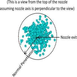
Normal Penetration (For nozzle-based analysis, variable name ends with '_NormalP (mm)')	[mm]	For the calculation, all spray parcels are projected onto the axis of the nozzle that injects them, and then the mass of these liquid parcels is accumulated starting at the axis of the nozzle. The normal penetration is defined as the normal distance between the nozzle axis and the location where the accumulated liquid mass reaches a threshold fraction of the total liquid mass specified by the "cutoff" parameter. It is a measure of spray diffusion away from the axis of injection.
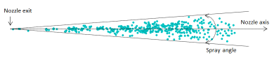
Spray Angle (For nozzle-based analysis, variable name ends with '_SprayAngle (deg)')	[degree]	For the calculation, all spray parcels are projected onto the axis of the nozzle that injects them, and then the mass of these liquid parcels is accumulated starting at the axis of the nozzle. For each spray parcel, a spreading angle can be defined by evaluating the ratio of its normal distance to the nozzle axis to its axial distance from the nozzle exit. A half-spray-cone angle is then defined where the accumulated liquid mass reaches a threshold fraction of the total liquid mass specified by the "cutoff" parameter. The spray angle reported doubles the half-spray-cone angle.
Injector Liquid Penetration (For injector-based analysis, variable name ends with '_LiqPene (mm)')	[mm]	Liquid penetration along a user-specified injector axis. The calculation method of this parameter is essentially the same as that of "Liquid penetration length" shown in Table 3.6: Spatially averaged variables that are always output to the .csv files for spray.csv, except that (1) the threshold fraction of the liquid mass is customizable instead of being fixed at 95%, and (2) the analysis is along the user-specified injector axis instead of a nozzle axis.
Injector Vapor Penetration (For injector-based analysis, variable name ends with '_VapPene (mm)')	[mm]	Vapor penetration along a user-specified injector axis. The calculation method of this parameter is essentially the same as that of "Vapor penetration length" shown in Table 3.6: Spatially averaged variables that are always output to the .csv files for spray.csv, except that (1) the threshold fraction of the vapor mass is customizable instead of being fixed at 99.9%, and (2) the analysis is along the user-specified injector axis instead of a nozzle axis.

Figure 3.25: Illustration of axial and radial penetrations (assuming the liquid mass threshold "cutoff" is 100%)

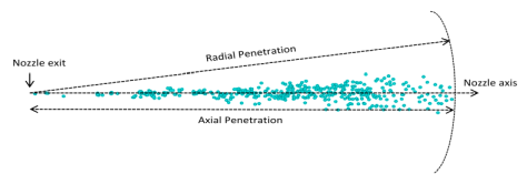
Figure 3.26: Illustration of normal penetration (assuming the liquid mass threshold "cutoff" is 100%)

Figure 3.27: Illustration of spray angle (assuming the liquid mass threshold "cutoff" is 100%)

3.7.2.7. Port Flow Monitor

In an engine system, it is often desirable to monitor the mass flow rate and accumulated mass flow through valves or ports between an engine cylinder and regions connected to it. The standard spatially averaged output flow_into_cylinder.csv reports these quantities, but it only reports the total mass flow through all the valves or ports that connect a cylinder region and a neighboring non-cylinder region. In practice, there may be more than one valve or port connecting the cylinder and the non-cylinder region. Port Flow Monitor can be used to monitor the mass flow through each individual valve/port or a selected group of valves/ports.

For each port flow monitor, you can select which valve(s)/port(s) to monitor by drawing either a bounding box or a bounding sphere that completely encompasses them. If the bounding box option is selected, a reference frame can be used to define the orientation of the box. The length, width, and height of the box are assumed to be aligned with the x, y, z-axes of the local reference frame. The specified location marks the center of the box. If the bounding sphere option is selected, the specified location marks the center of the sphere.

In a multicylinder simulation, if port flow monitors are used, an output file called port_flow_monitor_n.csv will be created for each cylinder, in which n corresponds to the cylinder index. Within each port_flow_monitor_n.csv, mass flow rate and accumulated mass flow through all the monitored valves/ports will be reported. The reported values follow the same sign convention as the one used by flow_into_cylinder.csv: positive if flow goes into the cylinder; negative if flow goes out of the cylinder.