


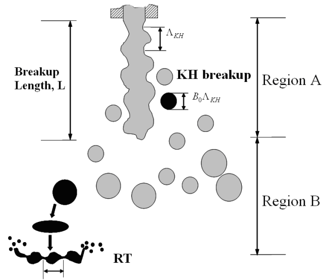
The spray atomization and droplet breakup of solid-cone sprays are modeled by the Kelvin-Helmholtz / Rayleigh-Taylor (KH /RT) hybrid breakup model [[11] , [90] ]. Figure 6.2: KH/RT breakup model for solid-cone sprays delineates the way the KH/RT breakup models are applied. The KH breakup model is applied within a specified Breakup Length, L , from the nozzle exit (region A). It strips small droplets off the jet (represented by parent parcels, or "blobs"), but the jet still maintains itself as a dense liquid core. Beyond the Breakup Length (region B), the RT model is used in conjunction with the KH model to predict secondary break-up [[102] , [11] ].
The Kelvin-Helmholtz (KH) model is based on linear stability analysis of a liquid jet [46] and is used to model the jet’s primary breakup [77] region. From the linear stability analysis any perturbation applied to a liquid-gas interface can be expanded as a Fourier series, with its fastest growing mode contributing to the eventual breakup and generation of new droplets. The growth rate and wave length of the fastest growing mode was found numerically [77] to be:
 | (6–20) |
 | (6–21) |
Here  is the wave length of the fastest growing wave,
  is its growth rate, r
p is the jet
radius,
is its growth rate, r
p is the jet
radius,  is surface tension, the dimensionless gas Weber number
We
g is defined as:
is surface tension, the dimensionless gas Weber number
We
g is defined as:
 | (6–22) |
with U rel being the magnitude of the liquid-gas relative velocity:
 | (6–23) |
Here  is the CFD gas-phase velocity,
  is the local gas-phase turbulent fluctuating velocity vector, and
  is the droplet velocity vector. Similarly, the liquid Weber number is defined
as:
is the droplet velocity vector. Similarly, the liquid Weber number is defined
as:
 | (6–24) |
and the dimensionless Ohnesorge number is:
 | (6–25) |
The Reynolds number is defined as:
 | (6–26) |
where  is the dynamic viscosity of the liquid. The last dimensionless number is the
Taylor number:
is the dynamic viscosity of the liquid. The last dimensionless number is the
Taylor number:
 | (6–27) |
The radius of new droplets (denoted as  ), which are created during the primary breakup process, is related to the
wave length
), which are created during the primary breakup process, is related to the
wave length  as follows:
 | (6–28) |
where  is the Size Constant of the KH breakup model.
Ansys Forte employs the concept of "blob injection" [78]
, in which the
liquid-jet injection is represented with parcels of blobs that have their initial
characteristic sizes equal to the effective nozzle diameter. Using this concept, primary
breakup is modeled as a process where new droplets (with radius  ) are formed from parent droplets (with radius
  ). The radius change of the parent droplet due to mass lost to its
"child" droplets is described by the rate equation [78]
:
). The radius change of the parent droplet due to mass lost to its
"child" droplets is described by the rate equation [78]
:
 | (6–29) |
where  is less than or equal to
  . Here, the breakup time scale
  is calculated as:
 | (6–30) |
In Equation 6–30
,  is the Time Constant of KH breakup. This is a user-controlled input for which
a general-purpose default value is provided in Ansys Forte.
is the Time Constant of KH breakup. This is a user-controlled input for which
a general-purpose default value is provided in Ansys Forte.
In general it is impractical to track each droplet formed from the parent droplet. Using the "droplets in parcel" concept, new droplets cannot leave their parent parcel until their mass reaches or exceeds 3% of the average injected parcel mass. The new droplets are then grouped into a "shed parcel" (or child parcel) that is separated from its parent. This parcel-shedding process helps to predict a realistic droplet size distribution in the primary breakup region. Also, as the number of parcels is increased, the local statistical resolution is improved. The value 3% is provided as a default model constant in Ansys Forte, which may be adjusted to change the size-distribution resolution.
Therefore, the KH breakup model involves two steps, as depicted in
Figure 6.3: Two-step approach in implementing the KH breakup model: the first step gradually reduces the parent droplet size
( ) by the rate equation (Equation 6–29
); the second step creates a new child
parcel from the parent, in which the child droplet size (
) by the rate equation (Equation 6–29
); the second step creates a new child
parcel from the parent, in which the child droplet size ( ) is predicted by Equation 6–28. The number of droplets in
the parent parcel is assumed to remain the same before and after the breakup, (that is:
) is predicted by Equation 6–28. The number of droplets in
the parent parcel is assumed to remain the same before and after the breakup, (that is:
 ).
).
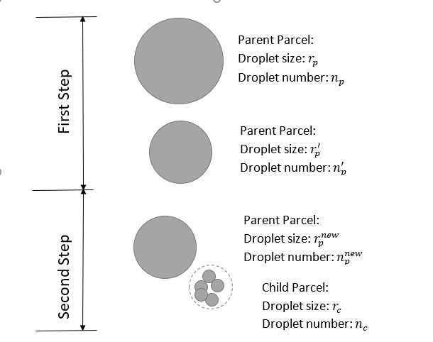
The problem remains to determine the droplet number in the child
parcel ( ), as well as the droplet size of the parent parcel (
 ). Two different options can be used:
In the first option, the droplet size in the parent parcel will remain the same when splitting with the child parcel, as
 . The droplet number of the child parcel is determined by mass conservation:
(6–31)
This is the default option used in Ansys Forte.
In the second option (activated by Impose SMR Conservation in KH Breakup), it is argued that the second breakup step is a numerical regrouping of droplets and is not an actual breakup event. The actual breakup event and the associated SMD reduction are already accounted for in the first breakup step, as governed by Equation 6–29. The splitting of the child parcel from the parent should not reduce the Sauter Mean Diameter (SMD) of the parent-child parcels, compared to the SMD of the parent parcel before the splitting. Therefore, in addition to mass conservation, the SMD of parent-child parcels is also conserved before and after the splitting. We solve Equation 6–32 and Equation 6–33:

(6–32)

(6–33)
These two equations can be combined into one equation for
 :
:
(6–34)
Equation 6–34 is solved by a Newton's iteration, which typically converges in 3 to 4 iterations. Once
 is obtained,
  is obtained from Equation 6–32.
 Imposing the SMD conservation constraint during child parcel splitting (Equation 6–33) typically leads to a slower breakup rate and larger SMD in the liquid core compared to the default option.
Beyond the Breakup Length from the nozzle exit, the Rayleigh-Taylor (RT) model is used together with the KH model to predict secondary breakup of spray droplets [[90] , [11] ]. The "breakup length" is defined in Levich's theory [46] as:
 | (6–35) |
in which  is a constant with value 10.29. The breakup length is implemented in Ansys Forte
as
is a constant with value 10.29. The breakup length is implemented in Ansys Forte
as
 | (6–36) |
in which  is nozzle diameter and
  is nozzle cross-sectional area,
  is set to 10.29, and
  is the RT Distance Constant exposed in the Ansys Forte interface. Compared to
Levich’s original definition Equation 6–35
,
is the RT Distance Constant exposed in the Ansys Forte interface. Compared to
Levich’s original definition Equation 6–35
,  in Equation 6–36
serves two purposes: one is a conversion factor from
in Equation 6–36
serves two purposes: one is a conversion factor from  to
to  ; the other is to serve as a knob for model calibration. The recommended value
for
; the other is to serve as a knob for model calibration. The recommended value
for  is approximately 1.9. The RT model is applied beyond the Breakup Length from
the nozzle exit.
is approximately 1.9. The RT model is applied beyond the Breakup Length from
the nozzle exit.
The RT model considers the instability generated when two fluids with different densities accelerate in a direction that is perpendicular to their interface. The frequency and wavelength of the fastest-growing wave are given by Bellman [12] as:
 | (6–37) |
 | (6–38) |
In the case of a high-speed droplet moving in air, a is the deceleration due to drag. As in the KH model, this fastest growing wave is assumed to lead to the breakup of droplets. The radius of the newly-formed droplet and the time of breakup are predicted as:
 | (6–39) |
 | (6–40) |
in which  ,
,  are two constants.
  is the Size Constant of RT Breakup.
  is the Time Constant of RT Breakup. Unlike the KH model, the standard
implementation of the RT model does not strip small child droplets off from their parent;
instead, a catastrophic breakup of the parent droplet into small droplets is assumed, and the
liquid column is eventually disintegrated and dispersed into the ambient gas.
is the Time Constant of RT Breakup. Unlike the KH model, the standard
implementation of the RT model does not strip small child droplets off from their parent;
instead, a catastrophic breakup of the parent droplet into small droplets is assumed, and the
liquid column is eventually disintegrated and dispersed into the ambient gas.
To reduce the time step dependency of the RT model, the RT breakup process is modeled by a rate equation similar to that of the KH model, Equation 6–29 :
 | (6–41) |
in which  is predicted by Equation 6–39
. The parent droplet breaks up
continuously at each time step, and the time-step dependency is avoided. Assuming
r
c and
is predicted by Equation 6–39
. The parent droplet breaks up
continuously at each time step, and the time-step dependency is avoided. Assuming
r
c and  does not change with time, Equation 6–41
can be solved analytically as:
does not change with time, Equation 6–41
can be solved analytically as:
 | (6–42) |
Here r
p,0 is the radius of
parent droplet at the start of break-up. Thus,  is the characteristic time required to break the parent droplet.
In practice, neither rate equation (Equation 6–29
) nor (Equation 6–41
) can be solved analytically, since both
r
c and  and (or
  ) change with time,
  and
and  can change significantly. Therefore, a sub-cycle approach is used to solve
these rate equations to eliminate time-step dependency.
can change significantly. Therefore, a sub-cycle approach is used to solve
these rate equations to eliminate time-step dependency.