


This tutorial describes how to use Ansys Forte CFD to simulate engine processes in an inline four-cylinder four-stroke spark-ignition engine. The purpose of this tutorial is to demonstrate several key points of project setup that are specific to multi-cylinder use cases:
Use (spatial) Reference Frames to facilitate the setup of location and orientation parameters in each cylinder.
Use Time Frames to facilitate the setup of timing parameters in each cylinder.
Approximate initial conditions in each cylinder region for a given starting crank angle.
Monitor output parameters that are averaged for each cylinder region.
Although the example used is an inline four-cylinder four-stroke spark-ignition engine, the concept and methodology described in this tutorial are also applicable to other multi-cylinder configurations, such as V-shaped arrangement, opposed piston engines, as well as other types of engine operations, such as spray combustion in diesel engines, HCCI, and others.
We recommend starting with the Ansys Forte Quick Start Guide , which explains the workflow of the Ansys Forte user interface, before doing this tutorial.
The files for this tutorial are obtained by downloading the
multicylinder_engine.zip file
here .
Unzip multicylinder_engine.zip to your working folder. The files
for this tutorial include:
multicylinder_4stroke_engine_tutorial.ftsim: A completely configured Ansys Forte project file.
intake_valve_lift_profile.csv: Lift profiles of the intake valves, tabulated for the crank angle range of [0, 720] °CA ATDC.
exhaust_valve_lift_profile.csv: Lift profiles of the exhaust valves, tabulated for the crank angle range of [0, 720] °CA ATDC.
multicylinder_4stroke_engine_tutorial.stl: An STL file that contains the multi-cylinder geometry. This is an optional file, which could be used as part of an exercise setting up this Ansys Forte project without using preconfigured files.
Note: This tutorial is based on a fully configured sample project that contains the tutorial project settings. The description provided here covers the key points of the project set-up but is not intended to explain every parameter setting in the project. The project files have all custom and default parameters already configured; the text highlights only the significant points of the tutorial. The tutorial assumes that the learner is already familiar with the fundamental steps for setting up a single-cylinder engine in Ansys Forte. Such prerequisite knowledge can be obtained by studying tutorials in previous chapters, such as the Ansys Forte GDI tutorial, Gasoline Direct Injection Engine Simulation.
Forte may be launched in a command line mode to perform certain tasks such as preparing a run for execution, importing project settings from a text file, or various other tasks described in the Forte User's Guide. One of these tools allows exporting a textual representation of the project data to a text file.
Example
forte.sh CLI -project <project_name>.ftsim -export tutorial_settings.txt
Briefly, you can double-check project settings by saving your project and then running the command-line utility to export the settings in your tutorial project (<project_name>.ftsim), and then use the command a second time to export the settings in the provided final version of the tutorial. Compare them with your favorite diff tool, such as DIFFzilla. If all the parameters are in agreement, you have set up the project successfully. If there are differences, you can go back into the tutorial set-up, re-read the tutorial instructions, and change the setting of interest.
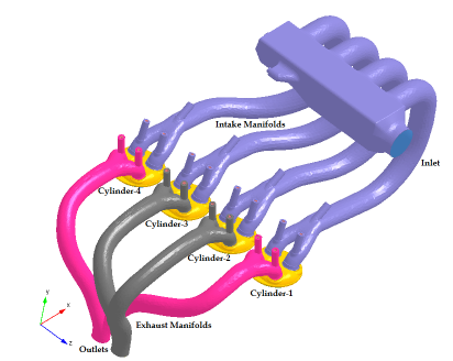
The configuration of the inline four-cylinder engine is shown in Figure 11.1: Configuration of the inline four-stroke multi-cylinder engine. The figure shows the numbering of the four cylinders, the intake manifolds merging at a plenum, the inlet located on the side of the plenum, as well as two groups of exhaust manifolds. One group of exhaust manifolds is connected to Cylinder-1 and Cylinder-4, the other is connected to Cylinder-2 and Cylinder-3. In this geometry, the crank shaft axis of the engine (not shown) is parallel to the Z-axis and the cylinder axes are parallel to the Y-axis. If you prefer, you can rotate the geometry so the cylinder axes are parallel to the z-axis. To do the rotation, select all the geometry surfaces under Geometry, right-click, select , and then select . The setup steps described below are based on the original orientation, not a transformed geometry. The engine geometry will serve as the surface mesh for the automatic mesh generation. Automatic Mesh Generation requires that all the pistons are positioned at their top-dead-center (TDC) location and all valves are at their closed location in the initial surface mesh.
There is one spark per cylinder central-mounted near the top of each cylinder head. The firing order of this engine is 1-3-4-2, which means that there is a 180 °CA phase delay between any two consecutive spark events.
In this tutorial, the fuel/air mixture preparation process inside the intake manifolds is simplified and no port fuel injection is simulated. Instead, the fuel and air are treated as premixed stoichiometric mixture, which enters the computational domain through the inlet connected to the plenum.
This section will go over the simulation setup steps, with emphasis on several aspects that are specific to multi-cylinder simulation.
Note: Time frames can be added under Geometry > Time Frames. However, the default state for the Time Frames node in the Workflow tree is hidden. To see it, use the command under on the ribbon or menu and check Enable Reference Time Frame Controls. Then Exit and restart Ansys Forte.
(Optional) If you wish to set up the case without using the preconfigured files, you can
start with importing the supplied STL geometry file. On the Geometry Editor
panel, click the Import Geometry![]() icon, and choose the Surface from one or more STL
files option, and then browse for the STL file. This step is needed only if you want
the exercise of setting up the case from scratch. These steps are not detailed here.
icon, and choose the Surface from one or more STL
files option, and then browse for the STL file. This step is needed only if you want
the exercise of setting up the case from scratch. These steps are not detailed here.
Reference frames and time frames in Ansys Forte allow you to define transforms to apply in space and time.
Reference frames used in Ansys Forte are spatially transformed coordinate systems. They can be defined in the Workflow tree under Geometry > Reference Frames. A new reference frame can be defined by referring to its parent coordinate system and through transformation of either or both the origin and orientation. In a multi-cylinder geometry, by defining equivalent local reference frames for all cylinders, you can use the same set of location and orientation parameters for all cylinders.
To make it convenient to set up equivalent local coordinate systems for all the cylinders, the geometry must meet some basic requirements relating to alignment with the coordinate axes in the global coordinate system. Generally, the minimum requirement is to let the crank shaft axis be parallel to one of the coordinate axes in the global coordinate. This tutorial case satisfies this requirement because its crank shaft axis is parallel to the Z-axis.
Now let us define a local reference frame for each cylinder. There are no fixed rules for setting the origin of each cylinder's own reference frame, but a convenient way is to use the center of the piston as the local origin. Using Cylinder-1 as an example, under Geometry, click surface piston_1. The piston_1 Editor panel shows the Min and Max coordinate values along X-, Y-, Z-directions in the global reference frame. The center of piston_1 on the X-Z plane can be calculated as
X_center = 0.5*(X_min + X_max) = 0.5*(-3.949 + 3.948) = 0 cm
Z_center = 0.5*(Z_min + Z_max) = 0.5* (31.15 + 39.05) = 35.1 cm
Since Y_min and Y_max are the same, you can pick Y_min as Y_center. In this specific example, it is beneficial to let all four cylinders have the same Y_center value.
In the fully configured .ftsim file, you can see four Reference Frames for the four cylinders: Frame-C1, Frame-C2, Frame-C3, and Frame-C4, listed in the Workflow tree. Their origins are calculated based on the method described above and the values are listed in Table 11.1: Origins of local reference frames for four cylinders. We can see that the distance along the Z-direction between the axes of two consecutive cylinders is 9.5 cm. These four reference frames do not involve orientation transformation. Orientation transformation is needed in a V-type multi-cylinder engine.
Table 11.1: Origins of local reference frames for four cylinders
| (cm) | Frame-C1 | Frame-C2 | Frame-C3 | Frame-C4 |
|---|---|---|---|---|
| Origin X | 0 | 0 | 0 | 0 |
| Origin Y | 19.7 | 19.7 | 19.7 | 19.7 |
| Origin Z | 35.1 | 25.6 | 16.1 | 6.6 |
In this tutorial engine, all the intake valves are tilted on the X-Y plane by -11° relative to the Y-axis, and all the exhaust valves are tilted in a similar manner, but by 12°. The tilt angles are illustrated in Figure 11.2: Tilt angles of intake and exhaust valve stems. Two reference frames are created for intake valves and exhaust valves, respectively, such that the Y-axes of these two reference frames are aligned with the moving directions of the valves. The names are Frame_Intake_Valves_Dir and Flame_Exhaust_Valves_Dir. The transformation only involves rotation about the Z-axis. These two reference frames can be used to define the moving directions of the valves. They can also be used to adjust the valve gaps at seated position if needed.

Note: If you cannot see Time Frames listed under Geometry in the Workflow tree, edit your Preferences as described in the note in Note early in this tutorial.
Time frames are convenient tools for managing all the timing parameters in a multi-cylinder context. A time frame requires input of a crank angle offset. An event associated with the time frame will be delayed by the offset value relative to the global crank angle. By defining an appropriate time frame for each cylinder, you can use the same set of timing parameters for all the cylinders in the configuration. Such timing parameters include, for example, piston motion specification and valve lift profiles, spark timing, and injection timing.
The Global Time is a prepopulated item, which corresponds to the global crank angle and serves as a reference. It cannot be edited. You can add four new time frames, one for each cylinder. Since the firing order of this engine is 1-3-4-2, the crank angle offset values can be set as 0 °CA, 180 °CA, 360 °CA, 540 °CA for Cylinder 1, 3, 4, 2, respectively. Note that Cylinder-1 is essentially associated with the global crank angle, and therefore it is used as a reference cylinder.
A multi-cylinder case requires that one of the cylinders be defined as the reference cylinder and associated with the Default Initialization region under Initial Conditions. The Material Point under Mesh Controls is expected to be a location inside the Default Initialization region. Since Cylinder-1 is assigned as the reference cylinder in this tutorial, the material point should be inside Cylinder-1. As mentioned earlier, since the origin of the reference frame for Cylinder-1 is defined as the center of the piston surface at the piston's TDC position, you can set the material point a distance above the local origin. The location selected should be able to remain inside the combustion chamber at all times while the piston travels from its BDC to TDC and the valves move from a fully closed position to a fully lifted position. In this sample, the Material Point is set to (X, Y, Z) = (0.0, 1.0, 0.0) cm in the Frame-C1 reference frame. The Global Mesh Size is set to 4.0 mm.
Several refinement controls for surface or volume are used to obtain higher mesh resolution at system boundaries and at various locations that are expected to see high gradients for velocity or temperature.
You can go through the refinement control items under Mesh Controls in the fully configured project file to check their detailed specifications.
Under Mesh Controls on the Workflow tree, AllWalls, OpenBoundaries, ValveStems, Chamber_BL, and ValveSeats are surface refinement controls that are applied at all times. ValveSeats specifies a 1/8 refinement for all valve seat surfaces in all the cylinders. In a typical engine geometry, cells near the valve gaps must be sufficiently refined (approximately 0.5 mm) to ensure that the computational domain of the intake/exhaust manifolds and the cylinders are cleanly separated when the corresponding valves are closed.
IVO_n and EVO_n, in which n is a numeral, are interval-based surface refinements applied to the combustion chamber walls during intake-valve opening or exhaust-valve opening processes. The cylinder-specific time frames are convenient when setting up these crank-angle-interval–based controls. By associating such a control with a cylinder's local time frame, you can specify the start angle and end angle values with respect to the cylinder's local TDC, and the same crank angle values can be used for all the cylinders. For example, the crank angle interval for refinement controls IVO_1 to IVO_4 has the same value, [323, 563] °CA ATDC. The only difference for this timing control is the time-frame selection. Note that the Location should point to the corresponding surfaces in each cylinder.
SparkPlug_1 to SparkPlug_4 are spherical volume refinement controls that specify 1/8 refinement in a small region surrounding each spark plug. The center of the refinement volume will be set at the spark location and the Radius of Application is 0.4 cm. By specifying the coordinates of the refinement center relative to the origin of each cylinder's local reference frame, the same center coordinates can be used for these four controls.
Note: As an option, you can limit this refinement to 10 °CA before spark and 60 °CA degree after spark in each cylinder.
Chemistry: The single-component 59-species gasoline chemical kinetics mechanism that is included in Ansys Forte's chemistry mechanism database is used to simulate the combustion of gasoline/air mixture, in which gasoline is approximated by iso-octane. The chemistry set can be found in the data folder within the Ansys Forte installation. The name of the chemistry set is Gasoline_1comp_49sp.cks.
Flame Speed Model: The Gülder formulation of the power law will be used to compute laminar flame speeds in the flame propagation model. For Unburned Calculation Method, the Volume Search with Variable Radius option will be used. For all the other model inputs on the Flame Speed Model panel, the default values are used.
Spark Ignition: Turn on the spark ignition model by checking the check box in front of Spark Ignition in the Workflow tree. On the Spark Ignition > Settings panel, the check box in front of Flame Propagation Model is checked by default. This means the flame propagation will be modeled using the discrete particle ignition kernel (DPIK) model and the G-equation model. Keep the default values for all the model constants.
Sparks: In this engine, each cylinder contains one spark
plug. The spark plug structure is included in the cylinder head surfaces. On the Spark Ignition Editor panel, you can create four spark plug items to
specify their location, spark duration, energy discharge rate, etc. Start with adding the spark
plug for the first cylinder by clicking the Spark  icon on the Spark Ignition Editor panel.
By specifying the spatial reference frame as Frame-C1, the coordinates of
the spark plug's location can be specified with respect to this cylinder's local
reference frame. The coordinates of the spark gap are (-0.4, 1.35, 0.0) cm.
Similarly, by linking this spark's timing parameter to Time Frame Cylinder
1, the spark timing value can be specified with respect to this cylinder's
local TDC. The spark timing is 20°CA before the firing TDC, so the starting angle of spark
is set to 700°CA ATDC. The default values are kept for spark energy
and initial kernel radius. After the first spark, Spark 1, has been
configured, you can then duplicate it (Copy
icon on the Spark Ignition Editor panel.
By specifying the spatial reference frame as Frame-C1, the coordinates of
the spark plug's location can be specified with respect to this cylinder's local
reference frame. The coordinates of the spark gap are (-0.4, 1.35, 0.0) cm.
Similarly, by linking this spark's timing parameter to Time Frame Cylinder
1, the spark timing value can be specified with respect to this cylinder's
local TDC. The spark timing is 20°CA before the firing TDC, so the starting angle of spark
is set to 700°CA ATDC. The default values are kept for spark energy
and initial kernel radius. After the first spark, Spark 1, has been
configured, you can then duplicate it (Copy ![]() and Paste
and Paste ![]() ) to create the spark plugs in the other three cylinders. After each copy
and paste, you can simply adjust the Time Frame and (spatial)
Reference Frame to their respective local frames.
) to create the spark plugs in the other three cylinders. After each copy
and paste, you can simply adjust the Time Frame and (spatial)
Reference Frame to their respective local frames.
Spray: (Optional) This tutorial does not involve spray simulation, but fuel sprays within each cylinder or within the intake ports of each cylinder could be set up in a similar manner as the spark setup. You can start with configuring the injector for the reference cylinder, and then duplicate that injector for the other cylinders. For each duplicated injector, you must adjust the time frame as well as the reference frames for each nozzle to use the cylinder's local frames. Note that the time frame is applied on the Injector level, that is, the injection timings of all the Injection pulses added under an injector are assumed to use the same time frame specified on the Injector Editor panel.
In the context of multi-cylinder engines, the boundary conditions can be divided into two groups, one is shared by all cylinders and the other is cylinder-specific. The cylinder-specific boundary conditions include head, liner, and moving surfaces (pistons and valves). For the cylinder-specific boundary conditions, you can first do the configuration for the reference cylinder, and then duplicate that for the rest of the cylinders. For each duplicated boundary condition item, the only parameters that must be adjusted are the Ref. Frames (for locations or directions) and Time Frames (for timings). Of course, the Location selection should be adjusted accordingly as well.
In this tutorial, boundary conditions shared by all the cylinders include Inlet, Outlet_1, Outlet_2, IntakeManifold, ExhaustManifold1, and ExhaustManifold2. The first three are open boundaries, which involve time profiles for boundary pressure and temperature. The time frame associated with these time profiles should be set to Global Time. In this tutorial, port fuel injection will not be simulated. Instead, the mixture coming into the domain through the inlet is assumed to be a premixed stoichiometric air/fuel mixture.
The boundary conditions head and liner are static wall boundaries. They are cylinder-specific, but do not require a time frame input, therefore the head surfaces of all cylinders are grouped as one boundary condition and the same is done for the liner surfaces. If preferred, you can split each group into four individual boundary condition items. Such a split may be needed if you want to define different wall boundary temperatures for different cylinders.
Each moving surface requires the specification of a Wall Motion. The wall motion for pistons and valves in different cylinders can easily be synchronized with the help of the cylinder-specific time frames. In the fully configured Ansys Forte project file, Piston_1, IntakeValve1-1, IntakeValve2-1, ExhaustValve1-1, ExhaustValve2-1 are the moving boundary conditions for Cylinder_1 (the last numeral in the BC name indicates the cylinder index). If setting up the project on your own, you could first create these five boundary conditions, specify the Time Frame as Cylinder 1, and specify the Ref. Frame used by the wall motion direction as Frame-C1. Then, duplicate these Boundary Conditions for the other cylinders.
For a duplicated piston, adjust three items to reflect the local cylinder:
Location selection;
TimeFrame; and
Ref. Frame (for motion direction).
For a duplicated valve, adjust four items:
Location selection;
Time Frame (for lift profiles);
Ref. Frame (for motion direction); and
the selection of Valve Seat and the Surface it Contacts.
All the other parameters can be kept the same for different cylinders, including the valve lift profiles.
Note that Frame-C1 to Frame-C4 are used to specify the valve motion direction in the current project file. An alternative (probably easier) way is to use the Ref. Frames mentioned earlier, Frame_Intake_Valves_Dir and Flame_Exhaust_Valves_Dir. For example, when using Frame_Intake_Valves_Dir to specify the moving direction of the intake valves, you can simply specify the Cartesian direction vector as (X, Y, Z) = (0, -1, 0). The same motion direction setting can be applied to all intake valves because they all move along the same direction. The same approach can be applied to the exhaust valves.
A multi-cylinder simulation should intrinsically also be a multi-cycle simulation. This is because the cylinders will be in different stages (strokes) of an engine cycle no matter where the simulation starts, and it will take multiple engine cycles to let the simulation reach a "converged" state starting from approximated initial conditions. Nonetheless, it is beneficial to provide a good estimate for initial conditions as this can help the simulation approach the "convergence" faster.
According to the lift profiles of the intake and exhaust valves and the minimum valve lift distance, the intake valves are open in crank angle interval [380, 580] °CA ATDC and the exhaust valves are open in [172, 380] °CA ATDC in each cylinder's local time frame. Thus, the firing TDC of this engine is 0°CA ATDC (or 720°CA ATDC). In this tutorial, we will set the starting crank angle to 0°CA ATDC. The starting angle is the global crank angle, which is also in sync with the local crank angle in Cylinder-1. At this starting angle, the piston positions and strokes each cylinder is about to start are listed in Table 11.2: Piston positions and strokes to begin in each cylinder:
Table 11.2: Piston positions and strokes to begin in each cylinder
| Piston Position | Stroke about to start | |
|---|---|---|
| Cylinder 1 | Firing TDC | Expansion/Work |
| Cylinder 2 | BDC (180° after Firing TDC) | Exhaust |
| Cylinder 3 | BDC (180° before Firing TDC) | Compression |
| Cylinder 4 | Non-Firing TDC | Intake |
Ansys Forte requires that the reference cylinder (Cylinder-1 in this case) be defined as the Default Initialization region. This default region will use the global material point for mesh creation and therefore does not require a separate material point input. In addition, the Region Type of the Default Initialization region is assumed to be Cylinder/Primary, and therefore it does not require a Region Type input.
Chamber-2, Chamber-3, and Chamber-4 are three new regions for the other three cylinders, and they are based on material points. By linking these regions to their respective spatial Ref. Frames, the material point coordinates can have the same value as the coordinates of the global material point. Note that the global Material Point under Mesh Controls in the Workflow tree is linked to Ref. Frame Frame-C1. For these three non-default cylinder regions, the Region Type should be specified as Cylinder/Primary. Note that the cylinder numbering will follow the order as they appear on the Workflow tree under Initial Conditions.
At the starting crank angle, Cylinder-1 is beginning the expansion stroke, the mixture is approximated as complete combustion products, the temperature and pressure are also approximated as peak values during combustion, 2000 K and 20 bar, respectively. Cylinder-2 is starting the exhaust stroke, so the composition is also set to complete combustion products, but the temperature and pressures are lower than those in Cylinder-1. They are set to 1200 K and 1.5 bar, respectively. Cylinder-3 is starting the compression stroke. Physically, the mixture inside this cylinder should be a fuel/air mixture mixed with a small fraction of residual gas. For simplicity, the initial composition is approximated as a stoichiometric fuel/air mixture. The temperature and pressure in Cylinder-3 should be similar to the values in the intake manifold. They are set to 340 K and 1 bar, respectively. Cylinder-4 is at the non-firing TDC and starting the intake stroke, the composition is mainly combustion products. The temperature and pressure are approximated as 600 K and 1 bar. The default settings are used in the fields for initial turbulence parameters and initial velocity.
Intake_Manifold, ExhaustManifold_1, and ExhaustManifold_2 are three regions with Region Type defined as Other. For Intake_Manifold, the initial composition is approximated as stoichiometric air/fuel mixture. Temperature and Pressure are set to 313.147 K and 1.1 bar, respectively. For the two exhaust ports, composition is set to combustion products, and Temperature and Pressure are set to 500 K and 1 bar, respectively. The material points can be placed anywhere inside the respective manifold geometry.
The Initialization Order values of all the initialization regions should be set following the "go-with-the-flow" rule. The order of the intake port should be 1, followed by the four cylinders, and finally the two exhaust manifolds.
The Composition Calculation Utility contained in the Ansys Forte Setup Interface can be used to prepare different mixtures required by the initial conditions.
A multi-cylinder engine simulation must use the Crank Angle Based option on the Simulation Controls Editor panel. The initial and final crank angles exposed on the Simulation Controls panel are both global values. In the fully configured project, the case is set up to run two complete engine cycles.
On the Time Step Editor panel, the Max Simulation Time Step, dtmax, uses a constant value (1.0E-5 s) in the current project. If a time varying dtmax profile is used instead, the profile is required to cover the crank angle range of [0, 720] °CA ATDC. This profile will be applied to all cylinders within each cylinder's local time frame. Specifically, a max time step value is first determined in each cylinder separately based on the profile and the cylinder's local crank angle value. Then, the minimum value among all the cylinders will be used as the global Max Simulation Time Step.
For the chemistry activation control on the Chemistry Solver panel, it is recommended not to check the After First Spark Event and After Fuel Injection Starts boxes because these controls are not well-defined in the multi-cycle, multi-cylinder context. Instead, you can use the During Crank Angle Interval option to activate chemistry for a certain duration within an engine cycle. Similar to the Max Simulation Time Step control, the interval-based chemistry activation control is also assumed to be applied in all the cylinders based on each cylinder's local time frame. For example, in this tutorial, the interval is set to [-40, 100] °CA ATDC. This means chemistry will be activated 40°CA before the Firing TDC and deactivated 100°CA after the Firing TDC in all four cylinders.
In a multi-cylinder calculation, cylinder-specific spatially-averaged solutions are reported on a per-cylinder basis. The cylinder-specific CSV output files include:
thermos.csv
dynamic.csv
flame.csv
massfraction.csv
molefraction.csv
speciesmass.csv
The cylinder index will be appended to the file names to indicate which cylinder they are for. For example, you will see thermo1.csv, thermo2.csv, etc. These files include both the global crank angle and the cylinder's local crank angle. The local crank angles are always converted to values within the range of [0, 720) °CA ATDC. For two-stroke engines, the local crank angles will be in the range of [0, 360) °CA ATDC.
The rest of the CSV files are reported either based on the average over the whole computational domain or reported on a per-boundary-condition basis, and they have the same format as single-cylinder calculations.